Perspectives on the Science
Evolving Standards for Resected High-Risk CSCC: Integrating Insights from C-POST and KEYNOTE-630
2025
Squamous Cell Carcinoma
Cemiplimab
Adjuvant
This perspective summarizes a multidisciplinary discussion of the C-POST trial, which demonstrated improved disease-free survival with adjuvant cemiplimab in patients with resected high-risk cutaneous squamous cell carcinoma (CSCC). Participants reflected on evolving practice patterns and considered the contrasting futility outcome of adjuvant pembrolizumab in the KEYNOTE-630 study. To help explore potential reasons for these divergent results, this piece incorporates reconstructed survival data—estimates derived from published Kaplan-Meier curves in the absence of individual patient data. The discussion underscores both the enthusiasm and the remaining uncertainty surrounding adjuvant immunotherapy in CSCC.
Vishal Anil Patel, MD 
Vernon Keith Sondak, MD
Vatche Tchekmedyian, MD
Ross David Merkin, MD
Isaac Brownell, MD, PhD
Reed E. Drews, MD
Sameer Gupta MD
Nikhil I. Khushalani, MD
Paul T. Nghiem, MD, PhD
Howard Lane Kaufman MD
Kevin Scott Emerick MD
Keywords
Squamous Cell Carcinoma, Cemiplimab, Adjuvant
Article status

Featured Article
Rischin, D. et al. Adjuvant Cemiplimab or Placebo in High-Risk Cutaneous Squamous-Cell Carcinoma. New England Journal of Medicine (2025).1
Introduction
On July 11, 2025, the Society of Cutaneous Oncology (SoCO) Journal Club convened to discuss a recent publication in the New England Journal of Medicine : “Adjuvant Cemiplimab or Placebo in High-Risk Cutaneous Squamous-Cell Carcinoma”1. The discussion brought together a multidisciplinary group of dermatologic, medical, and surgical oncologists—joined by colleagues from industry—to explore the evolving treatment landscape for CSCC (Figure 1).
Attendees included clinicians and researchers affiliated with institutions such as Massachusetts General Hospital, Massachusetts Eye and Ear Infirmary, University of Washington, Moffitt Cancer Center, Brigham and Women’s Hospital, Johns Hopkins Kimmel Cancer Center, University of North Carolina School of Medicine, Beth Israel Deaconess Medical Center, George Washington Cancer Center, Maine Health, the University of Texas, and the National Institutes of Health. Additional industry guests from Regeneron were invited.
Experience managing cutaneous squamous cell carcinoma varied across participants (Figure 2), which summarizes responses from academic respondents.
This perspective reviews major discussion points from the session, considering how the study’s findings may shape evolving approaches to the perioperative management of high-risk resectable CSCC. The views expressed here represent those of the authors and participants and do not necessarily represent official positions of the Society of Cutaneous Oncology or any affiliated institutions.
Background
Cutaneous squamous cell carcinoma is among the most common malignancies worldwide, and while most patients achieve cure with surgery alone, some subsets with high-risk features—such as nodal involvement or locally advanced primary tumors—faces a substantial risk of locoregional and distant recurrence despite surgery and radiotherapy2.
The introduction of PD-1 inhibitors transformed the treatment landscape for unresectable or metastatic CSCC, demonstrating high response rates and durable disease control3–10. Building on this success, a phase 2, multicenter study of neoadjuvant cemiplimab reported a pathological complete response in more than half of patients with resectable stage II–IV disease11,12—findings that have fueled enthusiasm for incorporating immunotherapy earlier in the course of treatment13,14.
Against this backdrop, the C-POST trial evaluated cemiplimab administered in the adjuvant setting after surgery and radiotherapy for patients at elevated risk of recurrence, aiming to determine whether postoperative immunotherapy in the absence of neoadjuvant anti-PD-1 therapy could further improve outcomes.
Even without formal regulatory approval in the adjuvant setting, many clinicians have already begun to explore the use of PD-1 inhibitors for high-risk resected CSCC in selected cases. In a pre-Journal Club survey of participants, more than half (64%) reported that they had personally recommended—or been part of a multidisciplinary team recommending—adjuvant anti-PD-1 therapy (Figure 3). This early adoption underscores both the perceived unmet need and the momentum behind immunotherapy integration across the disease continuum.
Study Design
C-POST is a multicenter, phase 3, randomized, double-blind, placebo-controlled trial evaluating adjuvant cemiplimab in patients with resectable cutaneous squamous cell carcinoma at highest risk for recurrence. Eligible patients had undergone complete surgical resection with curative intent with either clear margins or microscopic residual disease followed by adjuvant radiotherapy. Key high-risk features included both nodal and non-nodal characteristics such as nodal disease with extracapsular extension, multiple involved lymph nodes, tumors with cortical bone or skull base involvement, clinical or radiographic perineural invasion or recurrent lesions with additional adverse characteristics.
In the primary (hypothesis-testing) portion of the trial, patients were randomly assigned in a 1:1 ratio to receive adjuvant cemiplimab or placebo. Initially, the protocol specified cemiplimab 350 mg administered intravenously every three weeks (Q3W). A subsequent amendment revised the regimen to allow a switch to every six weeks (Q6W) after the initial induction period: cemiplimab 350 mg was given every three weeks for 12 weeks, followed by cemiplimab 700 mg every six weeks for an additional 36 weeks. Patients assigned to placebo received matching infusions on the same schedule. Treatment continued for up to 48 weeks or until disease recurrence, unacceptable toxicity, or withdrawal of consent.
The primary endpoint was disease-free survival (DFS), defined as the time from randomization to recurrence or death. Secondary endpoints assessed freedom from locoregional and distant recurrence, overall survival, the development of new primary cutaneous squamous-cell carcinoma tumors, and safety.
Main Findings
The trial met its primary endpoint, demonstrating a significant improvement in DFS in patients receiving adjuvant cemiplimab. At 24 months, 87.1% of patients receiving cemiplimab remained alive and free of disease recurrence compared with 64.1% in the placebo group. The hazard ratio for disease recurrence or death was 0.32 (95% CI, 0.20–0.51; p<0.001), and median DFS was not reached in the cemiplimab arm. Benefit was consistent across prespecified subgroups, including age, sex, anatomic site, ECOG performance status, and high-risk features such as nodal disease and perineural invasion.
Cemiplimab was also associated with a lower risk of locoregional and distant recurrence, with hazard ratios of 0.20 and 0.35, respectively.
Overall survival data remain immature. At the primary data cutoff, 25 deaths had been reported: 12 due to disease progression (4 in the cemiplimab group and 8 in the placebo group) and 13 due to other causes. Two-year overall survival was high in both groups—94.8% (95% CI, 89.6–97.4) with cemiplimab and 92.3% (95% CI, 86.5–95.7) with placebo—yielding a hazard ratio for death of 0.86 (95% CI, 0.39–1.90). Roughly half of the 51 placebo-treated patients who recurred went on to receive cemiplimab as subsequent therapy. At a later data cutoff in April 2025, 33 deaths had been reported overall (15 cemiplimab, 18 placebo), with a hazard ratio of 0.78 (95% CI, 0.39–1.56).
Safety findings were consistent with prior studies of PD-1 blockade. Grade 3 or higher adverse events occurred in 23.9% of patients receiving cemiplimab, including serious adverse events in 17.6% and treatment discontinuation in 9.8%. There were two deaths considered related to treatment in each study arm.
Overall, these results support the use of adjuvant cemiplimab as an effective strategy to reduce recurrence risk in patients with resected, locally advanced high-risk CSCC.
Discussion
Why This Study Matters
The study results come amid considerable uncertainty around the optimal management of patients with resectable high-risk CSCC. This is, in part, due to the success of immune checkpoint blockade for CSCC and the availability of neoadjuvant clinical data prior to adjuvant therapy data. Even before publication, many clinicians were grappling with complex, individualized treatment decisions that increasingly integrate immunotherapy in both preoperative and postoperative settings. This is exemplified by the diverse responses to our survey case vignette describing a 71-year-old patient with a parotid nodal metastasis. Although the majority favored an immunotherapy-first approach—either neoadjuvant PD-1 blockade or induction therapy with reassessment—others preferred immediate surgery, sometimes paired with postoperative radiotherapy or adjuvant systemic therapy (Figure 4). Such variability shows how, in the absence of a clear standard, multidisciplinary teams must navigate competing priorities of disease control, toxicity risk, and patient preference.
Dueling Trials, Divergent Reactions
At the same time, these discussions have been shaped by the strikingly divergent trajectories of the only two randomized trials conducted in this setting. In August 2024, Merck announced via press release that KEYNOTE-630—a similarly designed phase 3 study of adjuvant pembrolizumab—had been stopped early for futility. By contrast, in January 2025, Regeneron reported that C-POST had met its primary endpoint, demonstrating a 68% reduction in the risk of recurrence. The coexistence of a negative trial and a positive trial, evaluating different PD-1 inhibitors in nearly identical clinical scenarios, created both anticipation and confusion among the cutaneous oncology community as we awaited the full dataset. Understanding how C-POST achieved its robust results, and how these findings might integrate into an era increasingly defined by preoperative immunotherapy, is a central question raised by this publication.
Shifting Patterns in Perioperative Immunotherapy
The C-POST trial findings were published during a period when practice patterns for resectable high-risk CSCC are rapidly evolving. In the absence of prior phase 3 randomized trial data, treatment recommendations have primarily relied on retrospective studies, small phase 2 trials, institutional experience, and consensus guidelines, with occasional extrapolation from related diseases such as melanoma and Merkel cell carcinoma. Multidisciplinary teams have worked to balance the benefits of adjuvant radiotherapy and the emerging role of anti–PD-1 immunotherapy, including increasing interest in preoperative administration.
Pre–Journal Club survey responses (Figures 4–8) illustrate the variability in clinician comfort and approach to integrating immunotherapy into the perioperative setting. For example, in the same scenario (Figure 4), clinicians were divided among strategies prioritizing neoadjuvant immunotherapy, definitive systemic therapy, or conventional surgery and radiotherapy combinations. When asked about comfort in omitting adjuvant radiation in favor of anti–PD-1 monotherapy, responses were nearly evenly split between ambivalence, discomfort, and relative comfort, revealing persistent uncertainty (Figure 5). This ambivalence reflects not only the evolving role of systemic therapy but also the practical challenges clinicians face in making decisions about postoperative radiation in the absence of clear consensus. It is worth noting that C-POST incorporated adjuvant radiation in both study arms prior to randomization; as such, the efficacy of anti–PD-1 therapy without prior radiotherapy remains untested. These uncertainties about how best to combine or sequence therapies highlight the broader question of when, and for whom, adjuvant radiation itself should be used.
Uncertainty Around the Role of Radiation
Adjuvant RT is commonly used in patients with perineural invasion, positive margins, recurrent tumors, or nodal disease-especially with multiple involved nodes, large nodal metastases, or extranodal extension, yet its supporting evidence stems from retrospective studies, not randomized trials. For example, National Comprehensive Cancer Network (NCCN) guidelines recommend considering adjuvant radiation for high-risk or very high-risk CSCC, citing retrospective data suggesting it can reduce local and regional recurrence risk by as much as 50%15. To date, no randomized trials have directly compared adjuvant RT to observation after clear-margin resection, and the existing evidence has been mixed: TROG 05.01, the largest randomized trial in this space, did not demonstrate improved locoregional control or survival when chemoradiation was compared with radiotherapy alone, and did not address the efficacy of RT itself versus observation16. Other series, including analyses by Ruiz et al.17 and Kim et al.18, have failed to show a survival benefit in patients with negative margins.
To help address this uncertainty, emerging molecular tools—including a 40-gene expression profile (GEP)—have shown promise in identifying patients more likely to benefit from postoperative radiation, suggesting a potential path toward more individualized risk stratification19,20.
Sequencing Immunotherapy: Pre-op or Post-op?
Several participants noted that the positive disease-free survival signal from C-POST may further reinforce the consideration of adjuvant cemiplimab for patients with nodal involvement or extracapsular extension—particularly in scenarios where traditional adjuvant radiation carries significant morbidity or when patient preference favors systemic therapy. Others observed that adjuvant immunotherapy will inevitably become part of the conversation for patients who present after already undergoing definitive surgery by another provider, in whom preoperative immunotherapy was not incorporated into the initial management.
Reflecting the preference for earlier intervention, a substantial proportion of respondents reported that if anti–PD-1 therapy were approved for adjuvant use by the United States Food and Drug Administration (FDA), their main barrier to adopting it would be a preference to use neoadjuvant ICI instead (Figure 6). This tension—balancing the potential advantages of treating microscopic residual disease against the immunologic rationale for preoperative therapy—underscores the need for further data to guide sequencing decisions.
Taken together, this diversity of perspectives highlights the extent to which evolving evidence, limited prospective data on adjuvant radiation, and emerging biomarkers are all being interpreted through the lens of individual experience, institutional precedent, and patient preference—resulting in persistent heterogeneity even in the face of compelling trial evidence supporting adjuvant PD-1 blockade. While the C-POST trial offers the first phase 3 evidence supporting adjuvant immunotherapy, it does not fully resolve questions about optimal sequencing, the relative benefit compared with neoadjuvant approaches, or the appropriateness of omitting radiotherapy in otherwise radiation-eligible patients. Indeed, when clinicians were asked about their likely future practice patterns, nearly all anticipated recommending anti–PD-1 therapy more often in the neoadjuvant setting than in the adjuvant setting (Figure 7). The group acknowledged that while there is randomized data comparing neoadjuvant to adjuvant checkpoint blockade in melanoma, this data does not exist for patients with CSCC. However, some clinicians noted that another way to interpret and reconcile the debate of neoadjuvant vs. adjuvant therapy is to take solace in the fact that C-POST now offers robust evidence of the value in providing adjuvant therapy in patients who may have not been offered neoadjuvant therapy prior to surgery, or for those who were determined to have relevant risk factors identified only after surgery.
Balancing Overtreatment and Disease Control
Several discussants raised an important nuance: the risk of overtreatment. By definition, adjuvant immunotherapy exposes all eligible patients—including those who would never have developed recurrent disease—to potential toxicity and treatment burden. In C-POST, although cemiplimab markedly reduced the hazard of recurrence (HR 0.32), it is notable that even in the placebo group, 60.4% of patients remained disease free at three years. This means that for every 100 patients treated in the adjuvant setting, up to 60 may never have needed systemic therapy. Some participants proposed that close observation, with prompt initiation of anti–PD-1 therapy upon recurrence, could be a reasonable alternative for select individuals.
The rationale for immediate adjuvant treatment is rooted in the hypothesis that targeting microscopic residual disease is more effective than waiting until clinically apparent relapse. Yet, this premise is not conclusively proven. Experience in melanoma strongly uggests that neoadjuvant immunotherapy—administered when macroscopic disease is still present—may produce more robust and durable antitumor immunity than adjuvant therapy alone. Whether this biological advantage applies to CSCC remains unknown.
Although not a primary endpoint, overall survival did not differ significantly between arms in C-POST, albeit the data remain immature. This raises the possibility that delayed initiation of anti–PD-1 therapy after recurrence could still salvage many patients without compromising long-term outcomes. Survival follow-up on C-POST is ongoing and will help further characterize the durability of benefit with adjuvant cemiplimab in high-risk CSCC patients. At the same time, focusing on overall survival alone may overlook key nuances in this population. Many patients with advanced CSCC are older and have substantial comorbidities, making endpoints such as disease-specific survival and recurrence-free survival especially relevant as measures of therapeutic efficacy. Moreover, recurrences can be clinically morbid, difficult to manage, and associated with meaningful declines in quality of life. This is particularly true in CSCC, where a large proportion of tumors arise in the head and neck—locations where recurrence often necessitates additional surgery or radiation that may result in disfigurement, loss of function, and long-term morbidity. As such, reducing recurrence risk remains a critical goal, even if overall survival may ultimately remain unaffected.
Ultimately, as several clinicians noted, in the absence of a clear overall survival advantage for adjuvant therapy, decisions around immediate treatment versus observation hinge on individual patient preferences, risk tolerance, and the willingness of both patients and providers to accept the trade-offs of early systemic therapy for what may be modest absolute benefit. Looking ahead, complementary tools such as gene expression profiling (e.g., 40-GEP) or circulating tumor DNA (ctDNA) may offer additional guidance—helping to better stratify recurrence risk and identify patients most likely to benefit from perioperative systemic therapy.
These considerations—combined with uncertainty about optimal sequencing, the lack of mature survival data, and the cost implications of treating many patients who might never recur—help explain why clinicians remain divided on the best path forward.
Toward More Nuanced Decision-Making
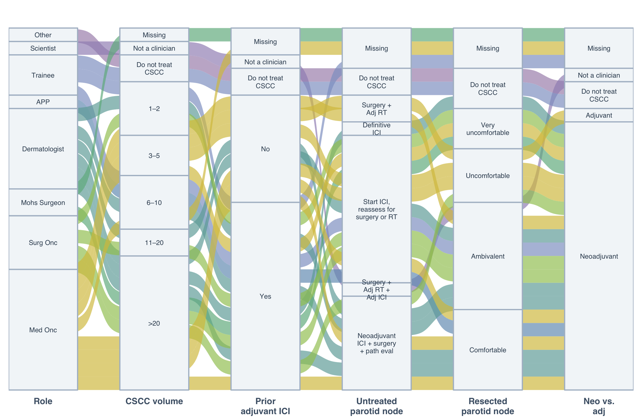
This diversity of perspectives is further illustrated in Figure 8, which maps how treatment decisions flow across clinician disciplines, experience levels, and preferred management strategies. Taken together, these data highlight how individual experience and institutional culture continue to shape practice—especially in a field where most evidence is retrospective or drawn from small, early-phase studies, and where the two available randomized trials yield conflicting results.
Reconciling C-POST and KEYNOTE-630
A Tale of Two Trials
One of the most intriguing questions arising from the publication of C-POST is why its results differ so substantially from those of KEYNOTE-630—two phase 3 trials testing adjuvant PD-1 inhibition in nearly identical clinical scenarios. While cemiplimab demonstrated a 68% reduction in recurrence risk in C-POST and is likely to establish adjuvant immunotherapy as a new standard for high-risk resectable CSCC, the contrasting futility outcome of KEYNOTE-630 adds complexity and raises questions about patient selection, trial design, and potential differences between the agents themselves.
Design, Dosing, and Treatment Initiation
Several hypotheses were raised during the Journal Club discussion. One possibility is that subtle but meaningful differences in eligibility criteria may have led to enrollment of patient populations with different prognostic risk profiles. As noted earlier and summarized in Table 1, C-POST included patients with a range of nodal and non-nodal high-risk features—including any nodal disease with extranodal extension, clinical or radiographic perineural invasion, or recurrent tumors meeting specific size and differentiation thresholds. Meanwhile, KEYNOTE-630 included many of the same criteria, but also some less clear or potentially less risky criteria such as an index tumor meeting at least two criteria of size, depth, or invasion as well as broader inclusion of patients with earlier and less numerous nodal disease without extranodal extension and microscopic perineural invasion. These nuances make direct comparison inherently challenging, but also can be interpreted as having identified the limited high-risk patients that may benefit most from adjuvant systemic immunotherapy.
To explore—not adjudicate—the apparent discordance between C-POST and KEYNOTE-630, we reconstructed pseudo–individual patient dataa (IPD) for recurrence-free survival from the published Kaplan–Meier curves of C-POST and the presented survival curves of KEYNOTE-630 (Figures 9–10). These reconstructions are necessarily approximate and permit only unadjusted, cross-trial descriptive comparisons; they cannot account for differences in eligibility, prognostic factors, endpoint ascertainment, follow-up, or other trial-level characteristics.
Within those limitations, the reconstructed placebo curves appeared broadly similar (Figure 9), with estimated 3-year recurrence-free survival around 60%. This provides no obvious signal that markedly different control-arm prognosis alone explains the divergent trial results, but it does not establish comparability between the study populations. The active-treatment curves remained notably different (Figure 10), with sustained separation for cemiplimab and substantially less separation for pembrolizumab. These observations are hypothesis-generating and should not be interpreted as a formal indirect comparison between cemiplimab and pembrolizumab.
NoteFigure 9. RFS in Placebo Arms of C-POST and KEYNOTE-630
Show Code for Placebo Arm IPD Reconstruction
#------------------------
# IPD for CPOST Placebo

# Load Packages
library(tidyverse)
library(survminer)
library(survival)
source(here::here("scripts", "save files.R"))

#--------------------------------------
# Number at risk at beginning is 206, Number of events in total 65, thus there 141 censored events
# Interval 0-4 months
# There are 45 events/censors from 206-161
## Maybe 19 events and 26 censors
# expected survival should drop from 100 to 89
# Set initial n and starting survival (adjust to your context)
initial_n <- 206
starting_survival <- 1

set.seed(123)
event_times1 <- 0.3
event_times2 <- 1.8
event_times3 <- c(2.0,2.0)
event_times4 <- runif(15, min = 2.1, max = 4.0)
event_times <- c(event_times1, event_times2, event_times3, event_times4)
df_events <- data.frame(
  time = event_times,
  status = 1
)
nrow(df_events)
# censoring
censor_times1 <- runif(2, min = 0.1, max = 0.1)
censor_times2 <- runif(24, min = 2.5, max = 2.8)
censor_times <- c(censor_times1, censor_times2)
df_censor <- data.frame(
  time = censor_times,
  status = 0
)
nrow(df_censor)

df_raw <- rbind(
  df_events,
  df_censor
)
nrow(df_raw)

# Sort
df_raw <- df_raw %>% arrange(time)

# Aggregate events and censorings
agg <- df_raw %>%
  group_by(time) %>%
  summarise(
    events = sum(status == 1),
    censored = sum(status == 0),
    .groups = "drop"
  ) %>%
  arrange(time)

print(agg)

# Prepare vectors
time_points <- agg$time
events <- agg$events
censored <- agg$censored

# Cumulative counts
cum_events <- cumsum(events)
cum_censored <- cumsum(censored)

# Compute risk sets
n_risk_start <- initial_n - c(0, head(cum_events + cum_censored, -1))

# Initialize storage vectors
decrements <- numeric(length(events))
cumulative_proportions <- numeric(length(events))
survival_estimates <- numeric(length(events))
hazard_increments <- numeric(length(events))
cumulative_hazard <- numeric(length(events))

# Loop over time points
current_survival <- 1
current_hazard <- 0

for (i in seq_along(events)) {
  n_risk_adj <- n_risk_start[i] - censored[i]
  if (n_risk_adj <= 0) stop("Risk set cannot be zero or negative after censoring.")

  decrement <- 1 - (events[i] / n_risk_adj)
  decrements[i] <- decrement

  current_survival <- current_survival * decrement
  cumulative_proportions[i] <- current_survival

  hazard_increment <- -log(decrement)
  hazard_increments[i] <- hazard_increment
  current_hazard <- current_hazard + hazard_increment
  cumulative_hazard[i] <- current_hazard

  survival_estimates[i] <- starting_survival * current_survival
}

# Combine into data frame
df <- data.frame(
  Time = time_points,
  Events = events,
  Censored = censored,
  Risk_Set_Start = n_risk_start,
  Risk_Set_Adjusted = n_risk_start - censored,
  Incremental_Decrement = round(decrements,4),
  Cumulative_Proportion = round(cumulative_proportions,4),
  Survival_Estimate = round(survival_estimates,4),
  Incremental_Hazard = round(hazard_increments,4),
  Cumulative_Hazard = round(cumulative_hazard,4)
)

# Add baseline row
baseline <- data.frame(
  Time = min(time_points) - 0.5,
  Events = 0,
  Censored = 0,
  Risk_Set_Start = NA,
  Risk_Set_Adjusted = NA,
  Incremental_Decrement = NA,
  Cumulative_Proportion = 1,
  Survival_Estimate = starting_survival,
  Incremental_Hazard = 0,
  Cumulative_Hazard = 0
)

# Combine
df_plot <- rbind(baseline, df)

# Review
print(df_plot)

df_interval_0_4 <- df_raw |> arrange(time)
nrow(df_interval_0_4)


#--------------------------------------
# Interval 4-8 months
# There are 31 events/censors from 161-130
## Maybe 13 events and 18 censors
# expected survival should drop from 88 to 72
# Set initial n and starting survival (adjust to your context)
initial_n <- 161
starting_survival <- 0.88

event_times1 <- 4.1
event_times2 <- runif(6, min = 4.4, max = 5.4)
event_times3 <- runif(6, min = 6.0, max = 7.5)
event_times <- c(event_times1, event_times2, event_times3)
df_events <- data.frame(
  time = event_times,
  status = 1
)
nrow(df_events)
# censoring
censor_times1 <- runif(17, min=4.7, max=5.4)
censor_times2 <- 6.0
censor_times <- c(censor_times1, censor_times2)

df_censor <- data.frame(
  time = censor_times,
  status = 0
)
nrow(df_censor)

df_raw <- rbind(
  df_events,
  df_censor
)

# Sort
df_raw <- df_raw %>% arrange(time)
nrow(df_raw)
# Aggregate events and censorings
agg <- df_raw %>%
  group_by(time) %>%
  summarise(
    events = sum(status == 1),
    censored = sum(status == 0),
    .groups = "drop"
  ) %>%
  arrange(time)

print(agg)

# Prepare vectors
time_points <- agg$time
events <- agg$events
censored <- agg$censored

# Cumulative counts
cum_events <- cumsum(events)
cum_censored <- cumsum(censored)

# Compute risk sets
n_risk_start <- initial_n - c(0, head(cum_events + cum_censored, -1))

# Initialize storage vectors
decrements <- numeric(length(events))
cumulative_proportions <- numeric(length(events))
survival_estimates <- numeric(length(events))
hazard_increments <- numeric(length(events))
cumulative_hazard <- numeric(length(events))

# Loop over time points
current_survival <- 1
current_hazard <- 0

for (i in seq_along(events)) {
  n_risk_adj <- n_risk_start[i] - censored[i]
  if (n_risk_adj <= 0) stop("Risk set cannot be zero or negative after censoring.")

  decrement <- 1 - (events[i] / n_risk_adj)
  decrements[i] <- decrement

  current_survival <- current_survival * decrement
  cumulative_proportions[i] <- current_survival

  hazard_increment <- -log(decrement)
  hazard_increments[i] <- hazard_increment
  current_hazard <- current_hazard + hazard_increment
  cumulative_hazard[i] <- current_hazard

  survival_estimates[i] <- starting_survival * current_survival
}

# Combine into data frame
df <- data.frame(
  Time = time_points,
  Events = events,
  Censored = censored,
  Risk_Set_Start = n_risk_start,
  Risk_Set_Adjusted = n_risk_start - censored,
  Incremental_Decrement = round(decrements,4),
  Cumulative_Proportion = round(cumulative_proportions,4),
  Survival_Estimate = round(survival_estimates,4),
  Incremental_Hazard = round(hazard_increments,4),
  Cumulative_Hazard = round(cumulative_hazard,4)
)

# Add baseline row
baseline <- data.frame(
  Time = min(time_points) - 0.5,
  Events = 0,
  Censored = 0,
  Risk_Set_Start = NA,
  Risk_Set_Adjusted = NA,
  Incremental_Decrement = NA,
  Cumulative_Proportion = 1,
  Survival_Estimate = starting_survival,
  Incremental_Hazard = 0,
  Cumulative_Hazard = 0
)

# Combine
df_plot <- rbind(baseline, df)

# Review
print(df_plot)


df_interval_4_8 <- df_raw |> arrange(time)
nrow(df_interval_4_8)
# Preview
head(df_interval_4_8, 10)

#--------------------------------------
# Interval 8-12
# There are 36 events/censors from 130-94
## 18 events and 18 censors
# expected survival should drop from 78 to 69.5
# Set initial n and starting survival (adjust to your context)
initial_n <- 130
starting_survival <- 0.78

event_times <- runif(18, min = 9, max = 11.8)
df_events <- data.frame(
  time = event_times,
  status = 1
  )
censor_times1 <- runif(9, min=8.1, max=8.9)
censor_times2 <- 8.9
censor_times3 <- runif(8, min = 10, max = 11.8)
censor_times <- c(censor_times1, censor_times2, censor_times3)

df_censor <- data.frame(
  time = censor_times,
  status = 0
)

df_raw <- rbind(
  df_events,
  df_censor
)
nrow(df_raw)
# Sort
df_raw <- df_raw %>% arrange(time)

# Aggregate events and censorings
agg <- df_raw %>%
  group_by(time) %>%
  summarise(
    events = sum(status == 1),
    censored = sum(status == 0),
    .groups = "drop"
  ) %>%
  arrange(time)

print(agg)

# Prepare vectors
time_points <- agg$time
events <- agg$events
censored <- agg$censored

# Cumulative counts
cum_events <- cumsum(events)
cum_censored <- cumsum(censored)

# Compute risk sets
n_risk_start <- initial_n - c(0, head(cum_events + cum_censored, -1))

# Initialize storage vectors
decrements <- numeric(length(events))
cumulative_proportions <- numeric(length(events))
survival_estimates <- numeric(length(events))
hazard_increments <- numeric(length(events))
cumulative_hazard <- numeric(length(events))

# Loop over time points
current_survival <- 1
current_hazard <- 0

for (i in seq_along(events)) {
  n_risk_adj <- n_risk_start[i] - censored[i]
  if (n_risk_adj <= 0) stop("Risk set cannot be zero or negative after censoring.")

  decrement <- 1 - (events[i] / n_risk_adj)
  decrements[i] <- decrement

  current_survival <- current_survival * decrement
  cumulative_proportions[i] <- current_survival

  hazard_increment <- -log(decrement)
  hazard_increments[i] <- hazard_increment
  current_hazard <- current_hazard + hazard_increment
  cumulative_hazard[i] <- current_hazard

  survival_estimates[i] <- starting_survival * current_survival
}

# Combine into data frame
df <- data.frame(
  Time = time_points,
  Events = events,
  Censored = censored,
  Risk_Set_Start = n_risk_start,
  Risk_Set_Adjusted = n_risk_start - censored,
  Incremental_Decrement = round(decrements,4),
  Cumulative_Proportion = round(cumulative_proportions,4),
  Survival_Estimate = round(survival_estimates,4),
  Incremental_Hazard = round(hazard_increments,4),
  Cumulative_Hazard = round(cumulative_hazard,4)
)

# Add baseline row
baseline <- data.frame(
  Time = min(time_points) - 0.5,
  Events = 0,
  Censored = 0,
  Risk_Set_Start = NA,
  Risk_Set_Adjusted = NA,
  Incremental_Decrement = NA,
  Cumulative_Proportion = 1,
  Survival_Estimate = starting_survival,
  Incremental_Hazard = 0,
  Cumulative_Hazard = 0
)

# Combine
df_plot <- rbind(baseline, df)

df_interval_8_12 <- df_raw |> arrange(time)
nrow(df_interval_8_12)

#--------------------------------------
# Interval from 12 - 16 months
# There are 12 events/censors from 94-82
## 2 events and 10 censors
# expected survival should drop from 69.5 to 67
# Assume initial number at risk
initial_n <- 94
starting_survival <- 0.695

event_times1 <- 13.4
event_times2 <- 14
event_times <- c(event_times1, event_times2)
df_events <- data.frame(
  time = event_times,
  status = 1
)
nrow(df_events)

# censoring
censor_times1 <- runif(10, min = 13.6, max = 15)
censor_times <- c(censor_times1)

df_censor <- data.frame(
  time = censor_times,
  status = 0
)
nrow(df_censor)

df_raw <- rbind(
  df_events,
  df_censor
)
nrow(df_raw)
# Sort
df_raw <- df_raw %>% arrange(time)

# Use dplyr to group and summarize
agg <- df_raw %>%
  group_by(time) %>%
  summarise(
    events = sum(status == 1),
    censored = sum(status == 0),
    .groups = "drop"
  ) %>%
  arrange(time)

print(agg)

# Expand counts
time_points <- agg$time
time_points
events <- agg$events
events
censored <- agg$censored
censored

cum_events <- cumsum(events)
cum_events
cum_censored <- cumsum(censored)
cum_censored

n_risk_start <- initial_n - c(0, head(cum_events + cum_censored, -1))
n_risk_start

print(data.frame(time=time_points, n_risk_start=n_risk_start, events=events, censored=censored))


# Initialize storage
decrements <- numeric(length(events))
decrements
cumulative_proportions <- numeric(length(events))
cumulative_proportions
survival_estimates <- numeric(length(events))
hazard_increments <- numeric(length(events))
cumulative_hazard <- numeric(length(events))

# Loop
current_survival <- 1
current_hazard <- 0

for (i in seq_along(events)) {
  n_risk_adj <- n_risk_start[i] - censored[i]

  if (n_risk_adj <= 0) stop("Risk set cannot be zero or negative after censoring.")

  decrement <- 1 - (events[i] / n_risk_adj)
  decrements[i] <- decrement

  current_survival <- current_survival * decrement
  cumulative_proportions[i] <- current_survival

  hazard_increment <- -log(decrement)
  hazard_increments[i] <- hazard_increment
  current_hazard <- current_hazard + hazard_increment
  cumulative_hazard[i] <- current_hazard

  survival_estimates[i] <- starting_survival * current_survival
}

# Create main data frame
df <- data.frame(
  Time = time_points,
  Events = events,
  Censored = censored,
  Risk_Set_Start = n_risk_start,
  Risk_Set_Adjusted = n_risk_start - censored,
  Incremental_Decrement = round(decrements,4),
  Cumulative_Proportion = round(cumulative_proportions,4),
  Survival_Estimate = round(survival_estimates,4),
  Incremental_Hazard = round(hazard_increments,4),
  Cumulative_Hazard = round(cumulative_hazard,4)
)

# Add baseline row
baseline <- data.frame(
  Time = min(time_points)-0.5,  # to show clearly before first event
  Events = 0,
  Censored = 0,
  Risk_Set_Start = NA,
  Risk_Set_Adjusted = NA,
  Incremental_Decrement = NA,
  Cumulative_Proportion = 1,
  Survival_Estimate = starting_survival,
  Incremental_Hazard = 0,
  Cumulative_Hazard = 0
)

# Combine
df_plot <- rbind(baseline, df)

# Build data frame
df_interval_12_16 <- df_raw |> arrange(time)

print(df_interval_12_16)

#--------------------------------------
# Interval from 16 - 20 months
# There are 13 events/censors from 82-69
## 2 events and 11 censors
# expected survival should drop from 68 to 67
# Assume initial number at risk
initial_n <- 82
starting_survival <- 0.68

event_times <- c(17, 18.5)
df_events <- data.frame(
  time = event_times,
  status = 1
)
nrow(df_events)

# censoring
censor_times1 <- runif(10, min=17.1, max=18.7)
censor_times2 <- 19.5
censor_times <- c(censor_times1, censor_times2)

df_censor <- data.frame(
  time = censor_times,
  status = 0
)
nrow(df_censor)

df_raw <- rbind(
  df_events,
  df_censor
)
nrow(df_raw)
# Sort
df_raw <- df_raw %>% arrange(time)

# Use dplyr to group and summarize
agg <- df_raw %>%
  group_by(time) %>%
  summarise(
    events = sum(status == 1),
    censored = sum(status == 0),
    .groups = "drop"
  ) %>%
  arrange(time)

print(agg)

# Expand counts
time_points <- agg$time
time_points
events <- agg$events
events
censored <- agg$censored
censored

cum_events <- cumsum(events)
cum_events
cum_censored <- cumsum(censored)
cum_censored

n_risk_start <- initial_n - c(0, head(cum_events + cum_censored, -1))
n_risk_start

print(data.frame(time=time_points, n_risk_start=n_risk_start, events=events, censored=censored))


# Initialize storage
decrements <- numeric(length(events))
decrements
cumulative_proportions <- numeric(length(events))
cumulative_proportions
survival_estimates <- numeric(length(events))
hazard_increments <- numeric(length(events))
cumulative_hazard <- numeric(length(events))

# Loop
current_survival <- 1
current_hazard <- 0

for (i in seq_along(events)) {
  n_risk_adj <- n_risk_start[i] - censored[i]

  if (n_risk_adj <= 0) stop("Risk set cannot be zero or negative after censoring.")

  decrement <- 1 - (events[i] / n_risk_adj)
  decrements[i] <- decrement

  current_survival <- current_survival * decrement
  cumulative_proportions[i] <- current_survival

  hazard_increment <- -log(decrement)
  hazard_increments[i] <- hazard_increment
  current_hazard <- current_hazard + hazard_increment
  cumulative_hazard[i] <- current_hazard

  survival_estimates[i] <- starting_survival * current_survival
}

# Create main data frame
df <- data.frame(
  Time = time_points,
  Events = events,
  Censored = censored,
  Risk_Set_Start = n_risk_start,
  Risk_Set_Adjusted = n_risk_start - censored,
  Incremental_Decrement = round(decrements,4),
  Cumulative_Proportion = round(cumulative_proportions,4),
  Survival_Estimate = round(survival_estimates,4),
  Incremental_Hazard = round(hazard_increments,4),
  Cumulative_Hazard = round(cumulative_hazard,4)
)

# Add baseline row
baseline <- data.frame(
  Time = min(time_points)-0.5,  # to show clearly before first event
  Events = 0,
  Censored = 0,
  Risk_Set_Start = NA,
  Risk_Set_Adjusted = NA,
  Incremental_Decrement = NA,
  Cumulative_Proportion = 1,
  Survival_Estimate = starting_survival,
  Incremental_Hazard = 0,
  Cumulative_Hazard = 0
)

# Combine
df_plot <- rbind(baseline, df)

# Check
print(df_plot)

# Build data frame
df_interval_16_20 <- df_raw |> arrange(time)


print(df_interval_16_20)

#--------------------------------------
# Interval 20-24
# There are 16 events/censors from 69-53
## 2 events and 14 censors
# expected survival should drop from 66 to 64.1
# Assume initial number at risk
initial_n <- 69
starting_survival <- 0.66

event_times <- c(21.5, 22)
df_events <- data.frame(
  time = event_times,
  status = 1
)
nrow(df_events)
# censoring
censor_times1 <- runif(10, min=20.5, max=22.1)
censor_times2 <- runif(4, min=23.1, max=23.8)
censor_times <- c(censor_times1, censor_times2)

df_censor <- data.frame(
  time = censor_times,
  status = 0
)
nrow(df_censor)

df_raw <- rbind(
  df_events,
  df_censor
)
nrow(df_raw)
# Sort
df_raw <- df_raw %>% arrange(time)

# Aggregate events and censorings
agg <- df_raw %>%
  group_by(time) %>%
  summarise(
    events = sum(status == 1),
    censored = sum(status == 0),
    .groups = "drop"
  ) %>%
  arrange(time)

print(agg)

# Prepare vectors
time_points <- agg$time
events <- agg$events
censored <- agg$censored

# Cumulative counts
cum_events <- cumsum(events)
cum_censored <- cumsum(censored)

# Compute risk sets
n_risk_start <- initial_n - c(0, head(cum_events + cum_censored, -1))

# Initialize storage vectors
decrements <- numeric(length(events))
cumulative_proportions <- numeric(length(events))
survival_estimates <- numeric(length(events))
hazard_increments <- numeric(length(events))
cumulative_hazard <- numeric(length(events))

# Loop over time points
current_survival <- 1
current_hazard <- 0

for (i in seq_along(events)) {
  n_risk_adj <- n_risk_start[i] - censored[i]
  if (n_risk_adj <= 0) stop("Risk set cannot be zero or negative after censoring.")

  decrement <- 1 - (events[i] / n_risk_adj)
  decrements[i] <- decrement

  current_survival <- current_survival * decrement
  cumulative_proportions[i] <- current_survival

  hazard_increment <- -log(decrement)
  hazard_increments[i] <- hazard_increment
  current_hazard <- current_hazard + hazard_increment
  cumulative_hazard[i] <- current_hazard

  survival_estimates[i] <- starting_survival * current_survival
}

# Combine into data frame
df <- data.frame(
  Time = time_points,
  Events = events,
  Censored = censored,
  Risk_Set_Start = n_risk_start,
  Risk_Set_Adjusted = n_risk_start - censored,
  Incremental_Decrement = round(decrements,4),
  Cumulative_Proportion = round(cumulative_proportions,4),
  Survival_Estimate = round(survival_estimates,4),
  Incremental_Hazard = round(hazard_increments,4),
  Cumulative_Hazard = round(cumulative_hazard,4)
)

# Add baseline row
baseline <- data.frame(
  Time = min(time_points) - 0.5,
  Events = 0,
  Censored = 0,
  Risk_Set_Start = NA,
  Risk_Set_Adjusted = NA,
  Incremental_Decrement = NA,
  Cumulative_Proportion = 1,
  Survival_Estimate = starting_survival,
  Incremental_Hazard = 0,
  Cumulative_Hazard = 0
)

# Combine
df_plot <- rbind(baseline, df)

df_interval_20_24 <- df_raw |> arrange(time)
nrow(df_interval_20_24)

#--------------------------------------
# Interval 24-28
# There are 11 events/censors from 53-42
## 1 events and 10 censors
# expected survival should drop from 64.1 to 62
# Assume initial number at risk
initial_n <- 53
starting_survival <- 0.641

event_times <- c(27.5)
df_events <- data.frame(
  time = event_times,
  status = 1
)
nrow(df_events)

# censoring
censor_times1 <- runif(9, min=24.9, max=27.2)
censor_times2 <- c(27.9)
censor_times <- c(censor_times1, censor_times2)

df_censor <- data.frame(
  time = censor_times,
  status = 0
)
nrow(df_censor)

df_raw <- rbind(
  df_events,
  df_censor
)
nrow(df_raw)
# Sort
df_raw <- df_raw %>% arrange(time)

# Aggregate events and censorings
agg <- df_raw %>%
  group_by(time) %>%
  summarise(
    events = sum(status == 1),
    censored = sum(status == 0),
    .groups = "drop"
  ) %>%
  arrange(time)

print(agg)

# Prepare vectors
time_points <- agg$time
events <- agg$events
censored <- agg$censored

# Cumulative counts
cum_events <- cumsum(events)
cum_censored <- cumsum(censored)

# Compute risk sets
n_risk_start <- initial_n - c(0, head(cum_events + cum_censored, -1))

# Initialize storage vectors
decrements <- numeric(length(events))
cumulative_proportions <- numeric(length(events))
survival_estimates <- numeric(length(events))
hazard_increments <- numeric(length(events))
cumulative_hazard <- numeric(length(events))

# Loop over time points
current_survival <- 1
current_hazard <- 0

for (i in seq_along(events)) {
  n_risk_adj <- n_risk_start[i] - censored[i]
  if (n_risk_adj <= 0) stop("Risk set cannot be zero or negative after censoring.")

  decrement <- 1 - (events[i] / n_risk_adj)
  decrements[i] <- decrement

  current_survival <- current_survival * decrement
  cumulative_proportions[i] <- current_survival

  hazard_increment <- -log(decrement)
  hazard_increments[i] <- hazard_increment
  current_hazard <- current_hazard + hazard_increment
  cumulative_hazard[i] <- current_hazard

  survival_estimates[i] <- starting_survival * current_survival
}

# Combine into data frame
df <- data.frame(
  Time = time_points,
  Events = events,
  Censored = censored,
  Risk_Set_Start = n_risk_start,
  Risk_Set_Adjusted = n_risk_start - censored,
  Incremental_Decrement = round(decrements,4),
  Cumulative_Proportion = round(cumulative_proportions,4),
  Survival_Estimate = round(survival_estimates,4),
  Incremental_Hazard = round(hazard_increments,4),
  Cumulative_Hazard = round(cumulative_hazard,4)
)

# Add baseline row
baseline <- data.frame(
  Time = min(time_points) - 0.5,
  Events = 0,
  Censored = 0,
  Risk_Set_Start = NA,
  Risk_Set_Adjusted = NA,
  Incremental_Decrement = NA,
  Cumulative_Proportion = 1,
  Survival_Estimate = starting_survival,
  Incremental_Hazard = 0,
  Cumulative_Hazard = 0
)

# Combine
df_plot <- rbind(baseline, df)

df_interval_24_28 <- df_raw |> arrange(time)
nrow(df_interval_24_28)

#--------------------------------------
# Interval 28-32
# There are 6 events/censors from 42-36
## 0 events and 6 censors
# expected survival should drop from 62-62
# Assume initial number at risk
initial_n <- 36
starting_survival <- 0.62

#event_times <- 30
#df_events <- data.frame(
#  time = event_times,
#  status = 1
#)

# censoring
censor_times1 <- runif(6, min=29, max=31.5)
#censor_times2 <- runif(6, min=30.1, max=31.6)
censor_times <- c(censor_times1)

df_censor <- data.frame(
  time = censor_times,
  status = 0
)
nrow(df_censor)

df_raw <-   df_censor
nrow(df_raw)
# Sort
df_raw <- df_raw %>% arrange(time)

df_interval_28_32 <- df_raw

print(df_interval_28_32)

#--------------------------------------
# Interval from 32 - 36 months
# There are 10 events/censors from 36-26
## 1 events and 9 censors
# expected survival should drop from 62 to 60.4
# Assume initial number at risk
initial_n <- 36
starting_survival <- 0.62

event_times <- c(34)
df_events <- data.frame(
  time = event_times,
  status = 1
)
nrow(df_events)
# censoring
censor_times1 <- runif(8, min=32.5, max=33.4)
censor_times2 <- 35
censor_times <- c(censor_times1, censor_times2)

df_censor <- data.frame(
  time = censor_times,
  status = 0
)
nrow(df_censor)

df_raw <- rbind(
  df_events,
  df_censor
  )

nrow(df_raw)

# Sort
df_raw <- df_raw %>% arrange(time)


# Aggregate events and censorings
agg <- df_raw %>%
  group_by(time) %>%
  summarise(
    events = sum(status == 1),
    censored = sum(status == 0),
    .groups = "drop"
  ) %>%
  arrange(time)

print(agg)

# Prepare vectors
time_points <- agg$time
events <- agg$events
censored <- agg$censored

# Cumulative counts
cum_events <- cumsum(events)
cum_censored <- cumsum(censored)

# Compute risk sets
n_risk_start <- initial_n - c(0, head(cum_events + cum_censored, -1))


# Initialize storage
decrements <- numeric(length(events))
cumulative_proportions <- numeric(length(events))
survival_estimates <- numeric(length(events))
hazard_increments <- numeric(length(events))
cumulative_hazard <- numeric(length(events))

# Loop
current_survival <- 1
current_hazard <- 0

for (i in seq_along(events)) {
  n_risk_adj <- n_risk_start[i] - censored[i]

  if (n_risk_adj <= 0) stop("Risk set cannot be zero or negative after censoring.")

  decrement <- 1 - (events[i] / n_risk_adj)
  decrements[i] <- decrement

  current_survival <- current_survival * decrement
  cumulative_proportions[i] <- current_survival

  hazard_increment <- -log(decrement)
  hazard_increments[i] <- hazard_increment
  current_hazard <- current_hazard + hazard_increment
  cumulative_hazard[i] <- current_hazard

  survival_estimates[i] <- starting_survival * current_survival
}

# Create main data frame
df <- data.frame(
  Time = time_points,
  Events = events,
  Censored = censored,
  Risk_Set_Start = n_risk_start,
  Risk_Set_Adjusted = n_risk_start - censored,
  Incremental_Decrement = round(decrements,4),
  Cumulative_Proportion = round(cumulative_proportions,4),
  Survival_Estimate = round(survival_estimates,4),
  Incremental_Hazard = round(hazard_increments,4),
  Cumulative_Hazard = round(cumulative_hazard,4)
)

# Add baseline row
baseline <- data.frame(
  Time = min(time_points)-0.5,  # to show clearly before first event
  Events = 0,
  Censored = 0,
  Risk_Set_Start = NA,
  Risk_Set_Adjusted = NA,
  Incremental_Decrement = NA,
  Cumulative_Proportion = 1,
  Survival_Estimate = starting_survival,
  Incremental_Hazard = 0,
  Cumulative_Hazard = 0
)

# Combine
df_plot <- rbind(baseline, df)

# Build data frame
df_interval_32_36 <- df_raw |> arrange(time)

print(df_interval_32_36)


#-----------------------------
# Interval from 36-60 months
# There are 26 events/censors from 26-0
## 2 events and 22 censors
# expected survival should drop from 60.4 to 48%
# Assume initial number at risk
initial_n <- 24
starting_survival <- 0.604

event_times <- c(48.5, 49.5)
df_events <- data.frame(
  time = event_times,
  status = 1
)
nrow(df_events)

# censoring
censor_times1 <- runif(2, min=36, max=40)
censor_times2 <- runif(6, min = 40.1, max = 44)
censor_times3 <- runif(8, min=44.1, max=48)
censor_times4 <- runif(2, min = 48.9, max = 49)
censor_times5 <- runif(2, min = 48.1, max = 52)
censor_times6 <- runif(2, min = 52.1, max = 56)
censor_times7 <- runif(2, min = 56.2, max = 58)
censor_times <- c(
  censor_times1, censor_times2, censor_times3, censor_times4, censor_times5, censor_times6, censor_times7
  )
df_censor <- data.frame(
  time = censor_times,
  status = 0
)
nrow(df_censor)

df_raw <-   rbind(
  df_events,
  df_censor
)
nrow(df_raw)
# Sort
df_raw <- df_raw %>% arrange(time)

df_interval_36_60 <- df_raw |> arrange(time)

print(df_interval_36_60)

#-------------------------
# Combine data frames
df_combined <- rbind(
  df_interval_0_4,
  df_interval_4_8,
  df_interval_8_12,
  df_interval_12_16,
  df_interval_16_20,
  df_interval_20_24,
  df_interval_24_28,
  df_interval_28_32,
  df_interval_32_36,
  df_interval_36_60
)

# Sort by time
df_combined <- df_combined |> arrange(time)

sum(df_combined$status)
nrow(df_combined)
sum(df_combined$status == 0)
# Inspect
print(head(df_combined, 10))

fit <- survfit(Surv(time, status) ~ 1, data = df_combined)
fit
summary(fit)$n.risk
summary(fit)$time

sumtab <- summary(fit)
df_sumtab <- data.frame(
  time = sumtab$time,
  n.risk = sumtab$n.risk,
  n.event = sumtab$n.event,
  n.censor = sumtab$n.censor,
  surv = sumtab$surv
)
ggsurv <- ggsurvplot(
  fit,
  conf.int = FALSE,
  risk.table = TRUE,
  xlab = "Time (Months)",
  ylab = "Estimated Survival Probability",
  break.time.by = 4,
  ggtheme = theme_minimal(base_size = 14),
  surv.scale = "percent"
)

print(ggsurv)
adjust_specific_times <- function(
    df,
    times,
    offsets,
    time_col = "time",
    tolerance = 1e-5
) {
  # Safety checks
  if (length(times) != length(offsets)) {
    stop("times and offsets must be the same length.")
  }

  df_new <- df

  # For tracking
  adjusted_rows <- list()

  for (i in seq_along(times)) {
    diffs <- abs(df_new[[time_col]] - times[i])
    idx <- which(diffs < tolerance)

    if (length(idx) == 0) {
      warning(sprintf(
        "Time %s not found within tolerance %g in %s column.",
        times[i], tolerance, time_col
      ))
    } else {
      df_new[idx, time_col] <- df_new[idx, time_col] + offsets[i]
      adjusted_rows[[i]] <- df_new[idx, ]
      message(sprintf(
        "Adjusted %d row(s) where %s approx. %s by %+g.",
        length(idx), time_col, times[i], offsets[i]
      ))
    }
  }

  return(df_new)
}
# adjust times to match number at risk
df_combined_adj <- adjust_specific_times(
  df = df_combined,
  times = c(
    15.202500, 23.987060),
  offsets = c(
    .8, .02
    )
)


fit_adj <- survfit(Surv(time, status) ~ 1, data = df_combined_adj)

ggsurv_adj <- ggsurvplot(
  fit_adj,
  conf.int = FALSE,
  risk.table = TRUE,
  xlab = "Time (Months)",
  ylab = "Estimated Survival Probability",
  break.time.by = 4,
  ggtheme = theme_minimal(base_size = 14),
  surv.scale = "percent",
  xlim = c(0, 60),          # Extend x-axis
  ylim = c(0, 1),           # Force y to 0–1
)

# Manually set y-axis breaks every 10%
ggsurv_adj$plot <- ggsurv_adj$plot +
  scale_y_continuous(
    labels = scales::percent_format(accuracy = 1),
    breaks = seq(0, 1, by = 0.1),
    limits = c(0, 1)
  )
print(ggsurv_adj)


save_files(
  save_object = df_combined_adj,
  filename = "CPOST Placebo Survival Table Reconstructed",
  subD = "files/reconstructed survival tables/CPOST/rfs/placebo",
  extension = ".csv"
)

# First, extract the ggplot object
p <- ggsurv_adj$plot

sumsurv <- summary(fit_adj, times = c(12, 24, 36))
surv_probs <- sumsurv$surv
surv_probs
surv_labels <- paste0(round(surv_probs * 100, 1), "%")

# Modify the internal ggplot object
ggsurv_adj$plot <- ggsurv_adj$plot +
  scale_y_continuous(
    labels = scales::percent_format(accuracy = 1),
    breaks = seq(0, 1, by = 0.1),
    limits = c(0, 1)
  ) +
  geom_vline(xintercept = c(12, 24, 36), linetype = "dashed", color = "black") +
  annotate(
    "text",
    x = c(12, 24, 36) + 0.75,
    y = surv_probs,
    label = surv_labels,
    color = "firebrick",
    size = 5,
    fontface = "bold",
    vjust = -0.5,
    hjust = 0
  )

# Print the *whole* ggsurvplot object
print(ggsurv_adj)

sum(df_combined$status)


#--------------------------
# IDP for KEYNOTE-630 IPD
# Load Packages
library(tidyverse)
library(survminer)
library(survival)
source(here::here("scripts", "save files.R"))

set.seed(123)
#--------------------------------------
# Interval 0-6 months
# There are 56 events/censors from 225-169
## Maybe 22 events and 35 censors
# expected survival should drop from 100 to 85.3

event_times0 <- c(0.4, 0.6)
event_times1 <- runif(5, min = 0.5, max = 2.0)
event_times2 <- runif(8, min = 2.9, max = 3.4)
event_times3 <-runif(4, min = 4, max = 4.9)
event_times4 <- runif(4, min = 5.3, max = 5.99)
event_times <- c(
  event_times0,
  event_times1, event_times2,
  event_times3, event_times4)
df_events <- data.frame(
  time = event_times,
  status = 1
)
nrow(df_events)

# censoring
censor_times1 <- runif(33, min=2.0, max=2.3)
censor_times2 <- runif(1, min=5.5, max=5.9)
censor_times3 <- 5.914729
censor_times <- c(censor_times1, censor_times2, censor_times3)

df_censor <- data.frame(
  time = censor_times,
  status = 0
)
nrow(df_censor)

df_raw <- rbind(
  df_events,
  df_censor
)
nrow(df_raw)

# Sort
df_raw <- df_raw %>% arrange(time)

# Aggregate events and censorings
agg <- df_raw %>%
  group_by(time) %>%
  summarise(
    events = sum(status == 1),
    censored = sum(status == 0),
    .groups = "drop"
  ) %>%
  arrange(time)

print(agg)

# Prepare vectors
time_points <- agg$time
events <- agg$events
censored <- agg$censored

# Set initial n and starting survival (adjust to your context)
initial_n <- 225
starting_survival <- 1

# Cumulative counts
cum_events <- cumsum(events)
cum_censored <- cumsum(censored)

# Compute risk sets
n_risk_start <- initial_n - c(0, head(cum_events + cum_censored, -1))

# Initialize storage vectors
decrements <- numeric(length(events))
cumulative_proportions <- numeric(length(events))
survival_estimates <- numeric(length(events))
hazard_increments <- numeric(length(events))
cumulative_hazard <- numeric(length(events))

# Loop over time points
current_survival <- 1
current_hazard <- 0

for (i in seq_along(events)) {
  n_risk_adj <- n_risk_start[i] - censored[i]
  if (n_risk_adj <= 0) stop("Risk set cannot be zero or negative after censoring.")

  decrement <- 1 - (events[i] / n_risk_adj)
  decrements[i] <- decrement

  current_survival <- current_survival * decrement
  cumulative_proportions[i] <- current_survival

  hazard_increment <- -log(decrement)
  hazard_increments[i] <- hazard_increment
  current_hazard <- current_hazard + hazard_increment
  cumulative_hazard[i] <- current_hazard

  survival_estimates[i] <- starting_survival * current_survival
}

# Combine into data frame
df <- data.frame(
  Time = time_points,
  Events = events,
  Censored = censored,
  Risk_Set_Start = n_risk_start,
  Risk_Set_Adjusted = n_risk_start - censored,
  Incremental_Decrement = round(decrements,4),
  Cumulative_Proportion = round(cumulative_proportions,4),
  Survival_Estimate = round(survival_estimates,4),
  Incremental_Hazard = round(hazard_increments,4),
  Cumulative_Hazard = round(cumulative_hazard,4)
)

# Add baseline row
baseline <- data.frame(
  Time = min(time_points) - 0.5,
  Events = 0,
  Censored = 0,
  Risk_Set_Start = NA,
  Risk_Set_Adjusted = NA,
  Incremental_Decrement = NA,
  Cumulative_Proportion = 1,
  Survival_Estimate = starting_survival,
  Incremental_Hazard = 0,
  Cumulative_Hazard = 0
)

# Combine
df_plot <- rbind(baseline, df)

# Review
print(df_plot)

ggplot(df_plot, aes(x = Time, y = Survival_Estimate)) +
  geom_step(color = "firebrick", size = 1.2, direction = "hv") +
  geom_point(aes(size = Events), color = "firebrick", alpha = 0.7) +
  geom_text(
    aes(
      label = ifelse(
        Events == 0 & Censored == 0,
        paste0("Start\nS=", round(Survival_Estimate,2)),
        paste0("E", Events, "\nC", Censored)
      )
    ),
    vjust = -1.2,
    size = 3.5
  ) +
  scale_y_continuous(labels = scales::percent_format(accuracy = 1)) +
  labs(
    title = "Stepwise Survival Estimate with Events and Censoring",
    x = "Time (Months)",
    y = "Estimated Survival Probability"
  ) +
  theme_minimal(base_size = 14)

df_interval_0_6 <- df_raw
nrow(df_interval_0_6)
# Sort by time for clarity
df_interval_0_6 <- df_interval_0_6[order(df_interval_0_6$time), ]
nrow(df_interval_0_6)
# Preview
head(df_interval_0_6, 10)


#--------------------------------------
# Interval 6-12 months
# There are 45 events/censors from 169-124
## Maybe 17 events and 28 censors
# expected survival should drop from 85.3 to 78.5

event_times1 <- 7
event_times2 <- runif(4, min = 8, max = 9)
event_times3 <- 9.5
event_times4 <- runif(10, min = 10, max = 11.95)
event_times <- c(event_times1, event_times2, event_times3, event_times4)
df_events <- data.frame(
  time = event_times,
  status = 1
)
nrow(df_events)
# censoring
censor_times0 <- runif(1, min=6.1, max=7)
censor_times1 <- runif(24, min=7.8, max=8.1)
censor_times2 <- 9.7
censor_times3 <- runif(1, min = 11.5, max = 11.6)
censor_times4 <- 11.835754
censor_times <- c(
  censor_times0,
  censor_times1, censor_times2, censor_times3, censor_times4)

df_censor <- data.frame(
  time = censor_times,
  status = 0
)
nrow(df_censor)

df_raw <- rbind(
  df_events,
  df_censor
)

# Sort
df_raw <- df_raw %>% arrange(time)

# Aggregate events and censorings
agg <- df_raw %>%
  group_by(time) %>%
  summarise(
    events = sum(status == 1),
    censored = sum(status == 0),
    .groups = "drop"
  ) %>%
  arrange(time)

print(agg)

# Prepare vectors
time_points <- agg$time
events <- agg$events
censored <- agg$censored

# Set initial n and starting survival (adjust to your context)
initial_n <- 169
starting_survival <- 0.853

# Cumulative counts
cum_events <- cumsum(events)
cum_censored <- cumsum(censored)

# Compute risk sets
n_risk_start <- initial_n - c(0, head(cum_events + cum_censored, -1))

# Initialize storage vectors
decrements <- numeric(length(events))
cumulative_proportions <- numeric(length(events))
survival_estimates <- numeric(length(events))
hazard_increments <- numeric(length(events))
cumulative_hazard <- numeric(length(events))

# Loop over time points
current_survival <- 1
current_hazard <- 0

for (i in seq_along(events)) {
  n_risk_adj <- n_risk_start[i] - censored[i]
  if (n_risk_adj <= 0) stop("Risk set cannot be zero or negative after censoring.")

  decrement <- 1 - (events[i] / n_risk_adj)
  decrements[i] <- decrement

  current_survival <- current_survival * decrement
  cumulative_proportions[i] <- current_survival

  hazard_increment <- -log(decrement)
  hazard_increments[i] <- hazard_increment
  current_hazard <- current_hazard + hazard_increment
  cumulative_hazard[i] <- current_hazard

  survival_estimates[i] <- starting_survival * current_survival
}

# Combine into data frame
df <- data.frame(
  Time = time_points,
  Events = events,
  Censored = censored,
  Risk_Set_Start = n_risk_start,
  Risk_Set_Adjusted = n_risk_start - censored,
  Incremental_Decrement = round(decrements,4),
  Cumulative_Proportion = round(cumulative_proportions,4),
  Survival_Estimate = round(survival_estimates,4),
  Incremental_Hazard = round(hazard_increments,4),
  Cumulative_Hazard = round(cumulative_hazard,4)
)

# Add baseline row
baseline <- data.frame(
  Time = min(time_points) - 0.5,
  Events = 0,
  Censored = 0,
  Risk_Set_Start = NA,
  Risk_Set_Adjusted = NA,
  Incremental_Decrement = NA,
  Cumulative_Proportion = 1,
  Survival_Estimate = starting_survival,
  Incremental_Hazard = 0,
  Cumulative_Hazard = 0
)

# Combine
df_plot <- rbind(baseline, df)

# Review
print(df_plot)

ggplot(df_plot, aes(x = Time, y = Survival_Estimate)) +
  geom_step(color = "firebrick", size = 1.2, direction = "hv") +
  geom_point(aes(size = Events), color = "firebrick", alpha = 0.7) +
  geom_text(
    aes(
      label = ifelse(
        Events == 0 & Censored == 0,
        paste0("Start\nS=", round(Survival_Estimate,2)),
        paste0("E", Events, "\nC", Censored)
      )
    ),
    vjust = -1.2,
    size = 3.5
  ) +
  scale_y_continuous(labels = scales::percent_format(accuracy = 1)) +
  labs(
    title = "Stepwise Survival Estimate with Events and Censoring",
    x = "Time (Months)",
    y = "Estimated Survival Probability"
  ) +
  theme_minimal(base_size = 14)

df_interval_6_12 <- df_raw
nrow(df_interval_6_12)
# Sort by time for clarity
df_interval_6_12 <- df_interval_6_12[order(df_interval_6_12$time), ]
nrow(df_interval_6_12)
# Preview
head(df_interval_6_12, 10)


#--------------------------------------
# Interval 12-18
# There are 23 events/censors from 124-101
## 9 events and 14 censors
# expected survival should drop from 78.5 to 72

event_times <- c(12.1, 12.2, 13, 14, 14.5, 15, 15.2, 16.5, 17.8) # n = 9
df_events <- data.frame(
  time = event_times,
  status = 1
)
censor_times1 <- runif(9, min=12.5, max = 12.9)
censor_times2 <- c(15.5, 15.6)
censor_times3 <- c(17.9, 17.9, 17.9)
censor_times <- c(censor_times1, censor_times2, censor_times3)

df_censor <- data.frame(
  time = censor_times,
  status = 0
)
nrow(df_censor)
df_raw <- rbind(
  df_events,
  df_censor
)

# Sort
df_raw <- df_raw %>% arrange(time)

# Aggregate events and censorings
agg <- df_raw %>%
  group_by(time) %>%
  summarise(
    events = sum(status == 1),
    censored = sum(status == 0),
    .groups = "drop"
  ) %>%
  arrange(time)

print(agg)

# Prepare vectors
time_points <- agg$time
events <- agg$events
censored <- agg$censored

# Set initial n and starting survival (adjust to your context)
initial_n <- 124
starting_survival <- 0.785

# Cumulative counts
cum_events <- cumsum(events)
cum_censored <- cumsum(censored)

# Compute risk sets
n_risk_start <- initial_n - c(0, head(cum_events + cum_censored, -1))

# Initialize storage vectors
decrements <- numeric(length(events))
cumulative_proportions <- numeric(length(events))
survival_estimates <- numeric(length(events))
hazard_increments <- numeric(length(events))
cumulative_hazard <- numeric(length(events))

# Loop over time points
current_survival <- 1
current_hazard <- 0

for (i in seq_along(events)) {
  n_risk_adj <- n_risk_start[i] - censored[i]
  if (n_risk_adj <= 0) stop("Risk set cannot be zero or negative after censoring.")

  decrement <- 1 - (events[i] / n_risk_adj)
  decrements[i] <- decrement

  current_survival <- current_survival * decrement
  cumulative_proportions[i] <- current_survival

  hazard_increment <- -log(decrement)
  hazard_increments[i] <- hazard_increment
  current_hazard <- current_hazard + hazard_increment
  cumulative_hazard[i] <- current_hazard

  survival_estimates[i] <- starting_survival * current_survival
}

# Combine into data frame
df <- data.frame(
  Time = time_points,
  Events = events,
  Censored = censored,
  Risk_Set_Start = n_risk_start,
  Risk_Set_Adjusted = n_risk_start - censored,
  Incremental_Decrement = round(decrements,4),
  Cumulative_Proportion = round(cumulative_proportions,4),
  Survival_Estimate = round(survival_estimates,4),
  Incremental_Hazard = round(hazard_increments,4),
  Cumulative_Hazard = round(cumulative_hazard,4)
)

# Add baseline row
baseline <- data.frame(
  Time = min(time_points) - 0.5,
  Events = 0,
  Censored = 0,
  Risk_Set_Start = NA,
  Risk_Set_Adjusted = NA,
  Incremental_Decrement = NA,
  Cumulative_Proportion = 1,
  Survival_Estimate = starting_survival,
  Incremental_Hazard = 0,
  Cumulative_Hazard = 0
)

# Combine
df_plot <- rbind(baseline, df)

# Review
print(df_plot)

ggplot(df_plot, aes(x = Time, y = Survival_Estimate)) +
  geom_step(color = "firebrick", size = 1.2, direction = "hv") +
  geom_point(aes(size = Events), color = "firebrick", alpha = 0.7) +
  geom_text(
    aes(
      label = ifelse(
        Events == 0 & Censored == 0,
        paste0("Start\nS=", round(Survival_Estimate,2)),
        paste0("E", Events, "\nC", Censored)
      )
    ),
    vjust = -1.2,
    size = 3.5
  ) +
  scale_y_continuous(labels = scales::percent_format(accuracy = 1)) +
  labs(
    title = "Stepwise Survival Estimate with Events and Censoring",
    x = "Time (Months)",
    y = "Estimated Survival Probability"
  ) +
  theme_minimal(base_size = 14)

df_interval_12_18 <- df_raw
nrow(df_interval_12_18)
# Sort by time for clarity
df_interval_12_18 <- df_interval_12_18[order(df_interval_12_18$time), ]
nrow(df_interval_12_18)
# Preview
head(df_interval_12_18, 10)


#--------------------------------------
# Interval from 18 - 24 months

# Assume initial number at risk
initial_n <- 101
starting_survival <- 0.72

# Recreate your raw data # 5 events and 16 censors
time <- c(
  18.1, #1 event
  18.5, #1 censor
  19.1, #1 event
  19.2, 19.3, 19.4, 19.5, 19.6, 20.9, # 6 censors
  21, #1 event,
  22,  #1 censor
  22.1,  #1 event
  22.2, 22.3, 22.4, #3 censors
  22.6, #1 event,
  22.7, 22.75, 23, 23.01, 23.5 #5 censors
  )
length(time)
status <- c(
  1,
  0,
  1,
  0,0,0,0,0,0, #6 censors
  1,
  0,
  1,
  0,0,0,
  1,
  0,0,0,0,0
)
length(status)


# Convert to data frame
df_raw <- data.frame(time=time, status=status)

# Use dplyr to group and summarize
agg <- df_raw %>%
  group_by(time) %>%
  summarise(
    events = sum(status == 1),
    censored = sum(status == 0),
    .groups = "drop"
  ) %>%
  arrange(time)

print(agg)

# Expand counts
time_points <- agg$time
time_points
events <- agg$events
events
censored <- agg$censored
censored

cum_events <- cumsum(events)
cum_events
cum_censored <- cumsum(censored)
cum_censored

n_risk_start <- initial_n - c(0, head(cum_events + cum_censored, -1))
n_risk_start

print(data.frame(time=time_points, n_risk_start=n_risk_start, events=events, censored=censored))


# Initialize storage
decrements <- numeric(length(events))
decrements
cumulative_proportions <- numeric(length(events))
cumulative_proportions
survival_estimates <- numeric(length(events))
hazard_increments <- numeric(length(events))
cumulative_hazard <- numeric(length(events))

# Loop
current_survival <- 1
current_hazard <- 0

for (i in seq_along(events)) {
  n_risk_adj <- n_risk_start[i] - censored[i]

  if (n_risk_adj <= 0) stop("Risk set cannot be zero or negative after censoring.")

  decrement <- 1 - (events[i] / n_risk_adj)
  decrements[i] <- decrement

  current_survival <- current_survival * decrement
  cumulative_proportions[i] <- current_survival

  hazard_increment <- -log(decrement)
  hazard_increments[i] <- hazard_increment
  current_hazard <- current_hazard + hazard_increment
  cumulative_hazard[i] <- current_hazard

  survival_estimates[i] <- starting_survival * current_survival
}

# Create main data frame
df <- data.frame(
  Time = time_points,
  Events = events,
  Censored = censored,
  Risk_Set_Start = n_risk_start,
  Risk_Set_Adjusted = n_risk_start - censored,
  Incremental_Decrement = round(decrements,4),
  Cumulative_Proportion = round(cumulative_proportions,4),
  Survival_Estimate = round(survival_estimates,4),
  Incremental_Hazard = round(hazard_increments,4),
  Cumulative_Hazard = round(cumulative_hazard,4)
)

# Add baseline row
baseline <- data.frame(
  Time = min(time_points)-0.5,  # to show clearly before first event
  Events = 0,
  Censored = 0,
  Risk_Set_Start = NA,
  Risk_Set_Adjusted = NA,
  Incremental_Decrement = NA,
  Cumulative_Proportion = 1,
  Survival_Estimate = starting_survival,
  Incremental_Hazard = 0,
  Cumulative_Hazard = 0
)

# Combine
df_plot <- rbind(baseline, df)

# Check
print(df_plot)


ggplot(df_plot, aes(x = Time, y = Survival_Estimate)) +
  geom_step(color = "firebrick", size = 1.2, direction = "hv") +
  geom_point(aes(size = Events), color = "firebrick", alpha = 0.7) +
  geom_text(
    aes(
      label = ifelse(
        Events == 0 & Censored == 0,
        paste0("Start\nS=", round(Survival_Estimate,2)),
        paste0("E", Events, "\nC", Censored)
      )
    ),
    vjust = -1.2,
    size = 3.5
  ) +
  scale_y_continuous(labels = scales::percent_format(accuracy = 1)) +
  labs(
    title = "Stepwise Survival Estimate with Events and Censoring",
    x = "Time (Months)",
    y = "Estimated Survival Probability"
  ) +
  theme_minimal(base_size = 14)


# Build data frame
df_interval_18_24 <- data.frame(
  time = time,
  status = status
)

print(df_interval_18_24)
#--------------------------------------
# Interval from 24 - 30 months
# 80-58, 4 events, 18 censors
# Survival should drop from 68.6 to 66
# Assume initial number at risk
initial_n <- 80
starting_survival <- 0.686
event_times <- c(24.5, 25, 28, 29)
df_events <- data.frame(
  time = event_times,
  status = 1
)
nrow(df_events)
# censoring
censor_times <- c(
  24.4,24.45,24.46,24.48,  #4 censored
  24.6,24.65,24.66,24.66,24.67,24.7,24.75,24.8,24.9,  #9 censored
  27,27.2,27.5,27.7,27.8  #5 censored
)
# Recreate your raw data
df_censor <- data.frame(
  time = censor_times,
  status = 0
)
nrow(df_censor)
# Convert to data frame
df_raw <- rbind(
  df_events,
  df_censor
)

# Use dplyr to group and summarize
agg <- df_raw %>%
  group_by(time) %>%
  summarise(
    events = sum(status == 1),
    censored = sum(status == 0),
    .groups = "drop"
  ) %>%
  arrange(time)

print(agg)

# Expand counts
time_points <- agg$time
time_points
events <- agg$events
events
censored <- agg$censored
censored

cum_events <- cumsum(events)
cum_events
cum_censored <- cumsum(censored)
cum_censored

n_risk_start <- initial_n - c(0, head(cum_events + cum_censored, -1))
n_risk_start

print(data.frame(time=time_points, n_risk_start=n_risk_start, events=events, censored=censored))


# Initialize storage
decrements <- numeric(length(events))
decrements
cumulative_proportions <- numeric(length(events))
cumulative_proportions
survival_estimates <- numeric(length(events))
hazard_increments <- numeric(length(events))
cumulative_hazard <- numeric(length(events))

# Loop
current_survival <- 1
current_hazard <- 0

for (i in seq_along(events)) {
  n_risk_adj <- n_risk_start[i] - censored[i]

  if (n_risk_adj <= 0) stop("Risk set cannot be zero or negative after censoring.")

  decrement <- 1 - (events[i] / n_risk_adj)
  decrements[i] <- decrement

  current_survival <- current_survival * decrement
  cumulative_proportions[i] <- current_survival

  hazard_increment <- -log(decrement)
  hazard_increments[i] <- hazard_increment
  current_hazard <- current_hazard + hazard_increment
  cumulative_hazard[i] <- current_hazard

  survival_estimates[i] <- starting_survival * current_survival
}

# Create main data frame
df <- data.frame(
  Time = time_points,
  Events = events,
  Censored = censored,
  Risk_Set_Start = n_risk_start,
  Risk_Set_Adjusted = n_risk_start - censored,
  Incremental_Decrement = round(decrements,4),
  Cumulative_Proportion = round(cumulative_proportions,4),
  Survival_Estimate = round(survival_estimates,4),
  Incremental_Hazard = round(hazard_increments,4),
  Cumulative_Hazard = round(cumulative_hazard,4)
)

# Add baseline row
baseline <- data.frame(
  Time = min(time_points)-0.5,  # to show clearly before first event
  Events = 0,
  Censored = 0,
  Risk_Set_Start = NA,
  Risk_Set_Adjusted = NA,
  Incremental_Decrement = NA,
  Cumulative_Proportion = 1,
  Survival_Estimate = starting_survival,
  Incremental_Hazard = 0,
  Cumulative_Hazard = 0
)

# Combine
df_plot <- rbind(baseline, df)

# Check
print(df_plot)


ggplot(df_plot, aes(x = Time, y = Survival_Estimate)) +
  geom_step(color = "firebrick", size = 1.2, direction = "hv") +
  geom_point(aes(size = Events), color = "firebrick", alpha = 0.7) +
  geom_text(
    aes(
      label = ifelse(
        Events == 0 & Censored == 0,
        paste0("Start\nS=", round(Survival_Estimate,2)),
        paste0("E", Events, "\nC", Censored)
      )
    ),
    vjust = -1.2,
    size = 3.5
  ) +
  scale_y_continuous(labels = scales::percent_format(accuracy = 1)) +
  labs(
    title = "Stepwise Survival Estimate with Events and Censoring",
    x = "Time (Months)",
    y = "Estimated Survival Probability"
  ) +
  theme_minimal(base_size = 14)


df_interval_24_30 <- df_raw
print(df_interval_24_30)

#--------------------------------------
# Interval 30-36
event_time <- 30.65
set.seed(1)
censor_time1 <- 30.6
censor_times <- runif(13, min=30.66, max=36)
length(censor_times)
time <- c(censor_time1, event_time, censor_times)
length(time)
status <- c(
  0,        # censor_time1
  1,        # event_time
  rep(0, length(censor_times))
)
length(status)

df_raw <- data.frame(
  time = time,
  status = status
)

# Sort
df_raw <- df_raw %>% arrange(time)

# Aggregate events and censorings
agg <- df_raw %>%
  group_by(time) %>%
  summarise(
    events = sum(status == 1),
    censored = sum(status == 0),
    .groups = "drop"
  ) %>%
  arrange(time)

print(agg)

# Prepare vectors
time_points <- agg$time
events <- agg$events
censored <- agg$censored

# Set initial n and starting survival (adjust to your context)
initial_n <- 58
starting_survival <- 0.642

# Cumulative counts
cum_events <- cumsum(events)
cum_censored <- cumsum(censored)

# Compute risk sets
n_risk_start <- initial_n - c(0, head(cum_events + cum_censored, -1))

# Initialize storage vectors
decrements <- numeric(length(events))
cumulative_proportions <- numeric(length(events))
survival_estimates <- numeric(length(events))
hazard_increments <- numeric(length(events))
cumulative_hazard <- numeric(length(events))

# Loop over time points
current_survival <- 1
current_hazard <- 0

for (i in seq_along(events)) {
  n_risk_adj <- n_risk_start[i] - censored[i]
  if (n_risk_adj <= 0) stop("Risk set cannot be zero or negative after censoring.")

  decrement <- 1 - (events[i] / n_risk_adj)
  decrements[i] <- decrement

  current_survival <- current_survival * decrement
  cumulative_proportions[i] <- current_survival

  hazard_increment <- -log(decrement)
  hazard_increments[i] <- hazard_increment
  current_hazard <- current_hazard + hazard_increment
  cumulative_hazard[i] <- current_hazard

  survival_estimates[i] <- starting_survival * current_survival
}

# Combine into data frame
df <- data.frame(
  Time = time_points,
  Events = events,
  Censored = censored,
  Risk_Set_Start = n_risk_start,
  Risk_Set_Adjusted = n_risk_start - censored,
  Incremental_Decrement = round(decrements,4),
  Cumulative_Proportion = round(cumulative_proportions,4),
  Survival_Estimate = round(survival_estimates,4),
  Incremental_Hazard = round(hazard_increments,4),
  Cumulative_Hazard = round(cumulative_hazard,4)
)

# Add baseline row
baseline <- data.frame(
  Time = min(time_points) - 0.5,
  Events = 0,
  Censored = 0,
  Risk_Set_Start = NA,
  Risk_Set_Adjusted = NA,
  Incremental_Decrement = NA,
  Cumulative_Proportion = 1,
  Survival_Estimate = starting_survival,
  Incremental_Hazard = 0,
  Cumulative_Hazard = 0
)

# Combine
df_plot <- rbind(baseline, df)

# Review
print(df_plot)

ggplot(df_plot, aes(x = Time, y = Survival_Estimate)) +
  geom_step(color = "firebrick", size = 1.2, direction = "hv") +
  geom_point(aes(size = Events), color = "firebrick", alpha = 0.7) +
  geom_text(
    aes(
      label = ifelse(
        Events == 0 & Censored == 0,
        paste0("Start\nS=", round(Survival_Estimate,2)),
        paste0("E", Events, "\nC", Censored)
      )
    ),
    vjust = -1.2,
    size = 3.5
  ) +
  scale_y_continuous(labels = scales::percent_format(accuracy = 1)) +
  labs(
    title = "Stepwise Survival Estimate with Events and Censoring",
    x = "Time (Months)",
    y = "Estimated Survival Probability"
  ) +
  theme_minimal(base_size = 14)

df_interval_30_36 <- data.frame(
  time = time,
  status = status
)
nrow(df_interval_30_36)
# Sort by time for clarity
df_interval_30_36 <- df_interval_30_36[order(df_interval_30_36$time), ]
nrow(df_interval_30_36)
# Preview
head(df_interval_30_36, 10)

#--------------------------------------
# Interval 36-42
set.seed(1)
censor_times <- runif(10, min=36.01, max=42)
status <- c(
  rep(0, length(censor_times))
)

df_interval_36_42 <- data.frame(
  time = censor_times ,
  status = status
)

# Sort by time for clarity
df_interval_36_42 <- df_interval_36_42[order(df_interval_36_42$time), ]

# Preview
head(df_interval_36_42, 10)

#--------------------------------------
# Interval 42-48
set.seed(1)
censor_times <- runif(17, min=42.01, max=48)
status <- c(
  rep(0, length(censor_times))
)

df_interval_42_48 <- data.frame(
  time = censor_times,
  status = status
)

# Sort by time for clarity
df_interval_42_48 <- df_interval_42_48[order(df_interval_42_48$time), ]

# Preview
head(df_interval_42_48, 10)


#--------------------------------------
# Interval from 48 - 54 months
# 9 events/censoring
# 3 events and 6 censors

# Example vectors
event_times <-  c(51.6, 52.0, 53.0)
df_events <- data.frame(
  time = event_times,
  status = 1
)
censored_times <- c(49.0, 49.01, 49.02, 49.1, 49.2, 49.21)
df_censor <- data.frame(
  time = censored_times,
  status = 0
)

df_raw <- rbind(
  df_events,
  df_censor
)

# Sort
df_raw <- df_raw %>% arrange(time)

# Aggregate events and censorings
agg <- df_raw %>%
  group_by(time) %>%
  summarise(
    events = sum(status == 1),
    censored = sum(status == 0),
    .groups = "drop"
  ) %>%
  arrange(time)

print(agg)

# Prepare vectors
time_points <- agg$time
events <- agg$events
censored <- agg$censored

# Set initial n and starting survival (adjust to your context)
initial_n <- 16
starting_survival <- 0.63

# Cumulative counts
cum_events <- cumsum(events)
cum_censored <- cumsum(censored)

# Compute risk sets
n_risk_start <- initial_n - c(0, head(cum_events + cum_censored, -1))


# Initialize storage
decrements <- numeric(length(events))
cumulative_proportions <- numeric(length(events))
survival_estimates <- numeric(length(events))
hazard_increments <- numeric(length(events))
cumulative_hazard <- numeric(length(events))

# Loop
current_survival <- 1
current_hazard <- 0

for (i in seq_along(events)) {
  n_risk_adj <- n_risk_start[i] - censored[i]

  if (n_risk_adj <= 0) stop("Risk set cannot be zero or negative after censoring.")

  decrement <- 1 - (events[i] / n_risk_adj)
  decrements[i] <- decrement

  current_survival <- current_survival * decrement
  cumulative_proportions[i] <- current_survival

  hazard_increment <- -log(decrement)
  hazard_increments[i] <- hazard_increment
  current_hazard <- current_hazard + hazard_increment
  cumulative_hazard[i] <- current_hazard

  survival_estimates[i] <- starting_survival * current_survival
}

# Create main data frame
df <- data.frame(
  Time = time_points,
  Events = events,
  Censored = censored,
  Risk_Set_Start = n_risk_start,
  Risk_Set_Adjusted = n_risk_start - censored,
  Incremental_Decrement = round(decrements,4),
  Cumulative_Proportion = round(cumulative_proportions,4),
  Survival_Estimate = round(survival_estimates,4),
  Incremental_Hazard = round(hazard_increments,4),
  Cumulative_Hazard = round(cumulative_hazard,4)
)

# Add baseline row
baseline <- data.frame(
  Time = min(time_points)-0.5,  # to show clearly before first event
  Events = 0,
  Censored = 0,
  Risk_Set_Start = NA,
  Risk_Set_Adjusted = NA,
  Incremental_Decrement = NA,
  Cumulative_Proportion = 1,
  Survival_Estimate = starting_survival,
  Incremental_Hazard = 0,
  Cumulative_Hazard = 0
)

# Combine
df_plot <- rbind(baseline, df)

# Check
print(df_plot)


ggplot(df_plot, aes(x = Time, y = Survival_Estimate)) +
  geom_step(color = "firebrick", size = 1.2, direction = "hv") +
  geom_point(aes(size = Events), color = "firebrick", alpha = 0.7) +
  geom_text(
    aes(
      label = ifelse(
        Events == 0 & Censored == 0,
        paste0("Start\nS=", round(Survival_Estimate,2)),
        paste0("E", Events, "\nC", Censored)
      )
    ),
    vjust = -1.2,
    size = 3.5
  ) +
  scale_y_continuous(labels = scales::percent_format(accuracy = 1)) +
  labs(
    title = "Stepwise Survival Estimate with Events and Censoring",
    x = "Time (Months)",
    y = "Estimated Survival Probability"
  ) +
  theme_minimal(base_size = 14)


# Build data frame
df_interval_48_54 <- df_raw

print(df_interval_48_54)


#-----------------------------
# Interval from 54 months

# Example vectors
events <-       c(0, 0, 0, 0, 0, 0, 0)
censored <-     c(0, 1, 1, 1, 1, 1, 1)
n_risk_start <- c(7, 7, 6, 5, 4, 3, 2)
time_points <-  c(54, 54.1, 55, 55.1, 55.2, 57.5, 60)  # <<-- your actual times
starting_survival <- 0.44

# Initialize storage
decrements <- numeric(length(events))
cumulative_proportions <- numeric(length(events))
survival_estimates <- numeric(length(events))
hazard_increments <- numeric(length(events))
cumulative_hazard <- numeric(length(events))

# Loop
current_survival <- 1
current_hazard <- 0

for (i in seq_along(events)) {
  n_risk_adj <- n_risk_start[i] - censored[i]

  if (n_risk_adj <= 0) stop("Risk set cannot be zero or negative after censoring.")

  decrement <- 1 - (events[i] / n_risk_adj)
  decrements[i] <- decrement

  current_survival <- current_survival * decrement
  cumulative_proportions[i] <- current_survival

  hazard_increment <- -log(decrement)
  hazard_increments[i] <- hazard_increment
  current_hazard <- current_hazard + hazard_increment
  cumulative_hazard[i] <- current_hazard

  survival_estimates[i] <- starting_survival * current_survival
}

# Create main data frame
df <- data.frame(
  Time = time_points,
  Events = events,
  Censored = censored,
  Risk_Set_Start = n_risk_start,
  Risk_Set_Adjusted = n_risk_start - censored,
  Incremental_Decrement = round(decrements,4),
  Cumulative_Proportion = round(cumulative_proportions,4),
  Survival_Estimate = round(survival_estimates,4),
  Incremental_Hazard = round(hazard_increments,4),
  Cumulative_Hazard = round(cumulative_hazard,4)
)

# Add baseline row
baseline <- data.frame(
  Time = min(time_points)-0.5,  # to show clearly before first event
  Events = 0,
  Censored = 0,
  Risk_Set_Start = NA,
  Risk_Set_Adjusted = NA,
  Incremental_Decrement = NA,
  Cumulative_Proportion = 1,
  Survival_Estimate = starting_survival,
  Incremental_Hazard = 0,
  Cumulative_Hazard = 0
)

# Combine
df_plot <- rbind(baseline, df)

# Check
print(df_plot)


ggplot(df_plot, aes(x = Time, y = Survival_Estimate)) +
  geom_step(color = "firebrick", size = 1.2, direction = "hv") +
  geom_point(aes(size = Events), color = "firebrick", alpha = 0.7) +
  geom_text(
    aes(
      label = ifelse(
        Events == 0 & Censored == 0,
        paste0("Start\nS=", round(Survival_Estimate,2)),
        paste0("E", Events, "\nC", Censored)
      )
    ),
    vjust = -1.2,
    size = 3.5
  ) +
  scale_y_continuous(labels = scales::percent_format(accuracy = 1)) +
  labs(
    title = "Stepwise Survival Estimate with Events and Censoring",
    x = "Time (Months)",
    y = "Estimated Survival Probability"
  ) +
  theme_minimal(base_size = 14)


# Interval 54 to 60
# Create vectors row by row
time <- c(
  54.1, 55, 55.1, 55.2, 57.5, 60   # 6 censorings

)

status <- c(
  0,0,0,0,0,0  # 6 censored
              # 0 events
)

# Build data frame
df_interval_54_60 <- data.frame(
  time = time,
  status = status
)

print(df_interval_54_60)

#-------------------------
# Combine data frames
df_combined <- rbind(
  df_interval_0_6,
  df_interval_6_12,
  df_interval_12_18,
  df_interval_18_24,
  df_interval_24_30,
  df_interval_30_36,
  df_interval_36_42,
  df_interval_42_48,
  df_interval_48_54,
  df_interval_54_60
)

# Sort by time
df_combined <- df_combined |> arrange(time)

sum(df_combined$status)
nrow(df_combined)
sum(df_combined$status == 0)
# Inspect
print(head(df_combined, 10))

fit <- survfit(Surv(time, status) ~ 1, data = df_combined)
fit
summary(fit)$n.risk
summary(fit)$time

sumtab <- summary(fit)
df_sumtab <- data.frame(
  time = sumtab$time,
  n.risk = sumtab$n.risk,
  n.event = sumtab$n.event,
  n.censor = sumtab$n.censor,
  surv = sumtab$surv
)
ggsurv <- ggsurvplot(
  fit,
  conf.int = FALSE,
  risk.table = TRUE,
  xlab = "Time (Months)",
  ylab = "Estimated Survival Probability",
  break.time.by = 6,
  ggtheme = theme_minimal(base_size = 14),
  surv.scale = "percent"
)

print(ggsurv)
adjust_specific_times <- function(
    df,
    times,
    offsets,
    time_col = "time",
    tolerance = 1e-5
) {
  # Safety checks
  if (length(times) != length(offsets)) {
    stop("times and offsets must be the same length.")
  }

  df_new <- df

  # For tracking
  adjusted_rows <- list()

  for (i in seq_along(times)) {
    diffs <- abs(df_new[[time_col]] - times[i])
    idx <- which(diffs < tolerance)

    if (length(idx) == 0) {
      warning(sprintf(
        "Time %s not found within tolerance %g in %s column.",
        times[i], tolerance, time_col
      ))
    } else {
      df_new[idx, time_col] <- df_new[idx, time_col] + offsets[i]
      adjusted_rows[[i]] <- df_new[idx, ]
      message(sprintf(
        "Adjusted %d row(s) where %s approx. %s by %+g.",
        length(idx), time_col, times[i], offsets[i]
      ))
    }
  }

  return(df_new)
}
# adjust times to match number at risk
df_combined_adj <- adjust_specific_times(
  df = df_combined,
  times = c(
    5.9147290,
    5.9137821, 11.835754,
    17.8, 23.5, 29, 35.704566, 41.668605,
    47.668605, 53.000000),
  offsets = c(
    0.1,
    0.1, .2,
    .3, .6, 1.1, 0.31, 0.5, 0.5, 1.1)
)


fit_adj <- survfit(Surv(time, status) ~ 1, data = df_combined_adj)

ggsurv_adj <- ggsurvplot(
  fit_adj,
  conf.int = FALSE,
  risk.table = TRUE,
  xlab = "Time (Months)",
  ylab = "Estimated Survival Probability",
  break.time.by = 6,
  ggtheme = theme_minimal(base_size = 14),
  surv.scale = "percent",
  xlim = c(0, 66),          # Extend x-axis
  ylim = c(0, 1),           # Force y to 0–1
)

sumsurv <- summary(fit_adj, times = c(12, 24, 36))
surv_probs <- sumsurv$surv
surv_probs
surv_labels <- paste0(round(surv_probs * 100, 1), "%")

# Modify the internal ggplot object
ggsurv_adj$plot <- ggsurv_adj$plot +
  scale_y_continuous(
    labels = scales::percent_format(accuracy = 1),
    breaks = seq(0, 1, by = 0.1),
    limits = c(0, 1)
  ) +
  geom_vline(xintercept = c(12, 24, 36), linetype = "dashed", color = "black") +
  annotate(
    "text",
    x = c(12, 24, 36) + 0.75,
    y = surv_probs,
    label = surv_labels,
    color = "firebrick",
    size = 5,
    fontface = "bold",
    vjust = -0.5,
    hjust = 0
  )

# Print the *whole* ggsurvplot object
print(ggsurv_adj)

save_files(
  save_object = df_combined_adj,
  filename = "KN630 RFS Placebo Survival Table Reconstructed",
  subD = "files/reconstructed survival tables/KN630/rfs/placebo",
  extension = ".csv"
)
sum(df_combined$status)
Reconstructed control-arm survival
The placebo arms tracked closely across trials.
Pseudo–individual patient data reconstructed from the published C-POST and presented KEYNOTE-630 recurrence-free survival curves.
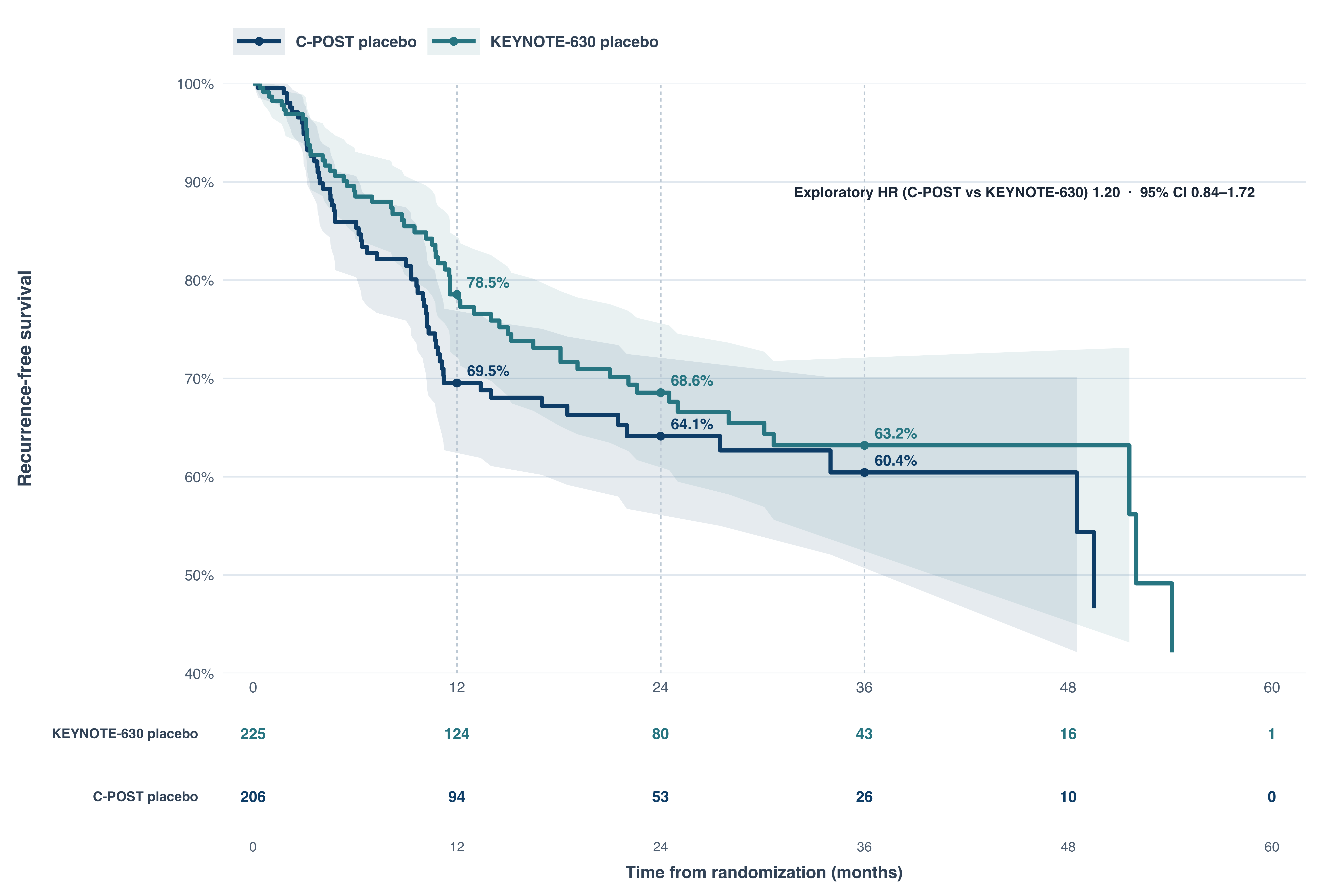
Figure 9. Reconstructed recurrence-free survival in the placebo arms of C-POST and KEYNOTE-630. Control-arm outcomes were broadly similar; the exploratory hazard ratio is derived from pseudo–individual patient data and should not be interpreted as a formal indirect treatment comparison.
NoteFigure 10. RFS Across Treatment Arms in C-POST and KEYNOTE-630
Show Code for Treatment Arm IPD Reconstruction
#--------------------------
# IPD from Cemiplimab treated patients in C-POST

# Load Packages
library(tidyverse)
library(survminer)
library(survival)
source(here::here("scripts", "save files.R"))

#--------------------------------------
# Number at risk at beginning is 209, Number of events in total 24, thus there 185 censored events
# Interval 0-4 months
# There are 37 events/censors from 209-172
## Maybe 9 events and 29 censors
# expected survival should drop from 100 to 90
# Set initial n and starting survival (adjust to your context)
initial_n <- 209
starting_survival <- 1
set.seed(123)
event_times1 <- runif(4, min = 0.53, max = 1.4)
event_times2 <- runif(4, min = 2, max = 2.9)
event_times3 <- 3.99
event_times <- c(event_times1, event_times2, event_times3)
df_events <- data.frame(
  time = event_times,
  status = 1
)
nrow(df_events)
# censoring
censor_times1 <- runif(8, min = 0.5, max = 0.51)
censor_times2 <- 3
censor_times3 <- runif(19, min = 3.1, max = 3.3)
censor_times <- c(censor_times1, censor_times2, censor_times3)

df_censor <- data.frame(
  time = censor_times,
  status = 0
)
nrow(df_censor)

df_raw <- rbind(
  df_events,
  df_censor
)
nrow(df_raw)

# Sort
df_raw <- df_raw %>% arrange(time)

# Aggregate events and censorings
agg <- df_raw %>%
  group_by(time) %>%
  summarise(
    events = sum(status == 1),
    censored = sum(status == 0),
    .groups = "drop"
  ) %>%
  arrange(time)

print(agg)

# Prepare vectors
time_points <- agg$time
events <- agg$events
censored <- agg$censored

# Cumulative counts
cum_events <- cumsum(events)
cum_censored <- cumsum(censored)

# Compute risk sets
n_risk_start <- initial_n - c(0, head(cum_events + cum_censored, -1))

# Initialize storage vectors
decrements <- numeric(length(events))
cumulative_proportions <- numeric(length(events))
survival_estimates <- numeric(length(events))
hazard_increments <- numeric(length(events))
cumulative_hazard <- numeric(length(events))

# Loop over time points
current_survival <- 1
current_hazard <- 0

for (i in seq_along(events)) {
  n_risk_adj <- n_risk_start[i] - censored[i]
  if (n_risk_adj <= 0) stop("Risk set cannot be zero or negative after censoring.")

  decrement <- 1 - (events[i] / n_risk_adj)
  decrements[i] <- decrement

  current_survival <- current_survival * decrement
  cumulative_proportions[i] <- current_survival

  hazard_increment <- -log(decrement)
  hazard_increments[i] <- hazard_increment
  current_hazard <- current_hazard + hazard_increment
  cumulative_hazard[i] <- current_hazard

  survival_estimates[i] <- starting_survival * current_survival
}

# Combine into data frame
df <- data.frame(
  Time = time_points,
  Events = events,
  Censored = censored,
  Risk_Set_Start = n_risk_start,
  Risk_Set_Adjusted = n_risk_start - censored,
  Incremental_Decrement = round(decrements,4),
  Cumulative_Proportion = round(cumulative_proportions,4),
  Survival_Estimate = round(survival_estimates,4),
  Incremental_Hazard = round(hazard_increments,4),
  Cumulative_Hazard = round(cumulative_hazard,4)
)

# Add baseline row
baseline <- data.frame(
  Time = min(time_points) - 0.5,
  Events = 0,
  Censored = 0,
  Risk_Set_Start = NA,
  Risk_Set_Adjusted = NA,
  Incremental_Decrement = NA,
  Cumulative_Proportion = 1,
  Survival_Estimate = starting_survival,
  Incremental_Hazard = 0,
  Cumulative_Hazard = 0
)

# Combine
df_plot <- rbind(baseline, df)

# Review
print(df_plot)

ggplot(df_plot, aes(x = Time, y = Survival_Estimate)) +
  geom_step(color = "firebrick", size = 1.2, direction = "hv") +
  geom_point(aes(size = Events), color = "firebrick", alpha = 0.7) +
  geom_text(
    aes(
      label = ifelse(
        Events == 0 & Censored == 0,
        paste0("Start\nS=", round(Survival_Estimate,2)),
        paste0("E", Events, "\nC", Censored)
      )
    ),
    vjust = -1.2,
    size = 3.5
  ) +
  scale_y_continuous(labels = scales::percent_format(accuracy = 1)) +
  labs(
    title = "Stepwise Survival Estimate with Events and Censoring",
    x = "Time (Months)",
    y = "Estimated Survival Probability"
  ) +
  theme_minimal(base_size = 14)

df_interval_0_4 <- df_raw
nrow(df_interval_0_4)
# Sort by time for clarity
df_interval_0_4 <- df_interval_0_4 |> arrange(time)
nrow(df_interval_0_4)
# Preview
head(df_interval_0_4, 10)

#--------------------------------------
# Interval 4-8 months
# There are 15 events/censors from 172-157
## Maybe 4 events and 11 censors
# expected survival should drop from 97-95.5
# Set initial n and starting survival (adjust to your context)
initial_n <- 172
starting_survival <- 0.97
event_times1 <- c(5.4, 5.8)
event_times2 <- c(6.8, 7.0)
event_times <- c(event_times1, event_times2)
df_events <- data.frame(
  time = event_times,
  status = 1
)
nrow(df_events)
# censoring
censor_times1 <- runif(10, min=5.0, max=6.0)
censor_times2 <- 7.8
censor_times <- c(censor_times1, censor_times2)

df_censor <- data.frame(
  time = censor_times,
  status = 0
)
nrow(df_censor)

df_raw <- rbind(
  df_events,
  df_censor
)

# Sort
df_raw <- df_raw %>% arrange(time)
nrow(df_raw)
# Aggregate events and censorings
agg <- df_raw %>%
  group_by(time) %>%
  summarise(
    events = sum(status == 1),
    censored = sum(status == 0),
    .groups = "drop"
  ) %>%
  arrange(time)

print(agg)

# Prepare vectors
time_points <- agg$time
events <- agg$events
censored <- agg$censored

# Cumulative counts
cum_events <- cumsum(events)
cum_censored <- cumsum(censored)

# Compute risk sets
n_risk_start <- initial_n - c(0, head(cum_events + cum_censored, -1))

# Initialize storage vectors
decrements <- numeric(length(events))
cumulative_proportions <- numeric(length(events))
survival_estimates <- numeric(length(events))
hazard_increments <- numeric(length(events))
cumulative_hazard <- numeric(length(events))

# Loop over time points
current_survival <- 1
current_hazard <- 0

for (i in seq_along(events)) {
  n_risk_adj <- n_risk_start[i] - censored[i]
  if (n_risk_adj <= 0) stop("Risk set cannot be zero or negative after censoring.")

  decrement <- 1 - (events[i] / n_risk_adj)
  decrements[i] <- decrement

  current_survival <- current_survival * decrement
  cumulative_proportions[i] <- current_survival

  hazard_increment <- -log(decrement)
  hazard_increments[i] <- hazard_increment
  current_hazard <- current_hazard + hazard_increment
  cumulative_hazard[i] <- current_hazard

  survival_estimates[i] <- starting_survival * current_survival
}

# Combine into data frame
df <- data.frame(
  Time = time_points,
  Events = events,
  Censored = censored,
  Risk_Set_Start = n_risk_start,
  Risk_Set_Adjusted = n_risk_start - censored,
  Incremental_Decrement = round(decrements,4),
  Cumulative_Proportion = round(cumulative_proportions,4),
  Survival_Estimate = round(survival_estimates,4),
  Incremental_Hazard = round(hazard_increments,4),
  Cumulative_Hazard = round(cumulative_hazard,4)
)

# Add baseline row
baseline <- data.frame(
  Time = min(time_points) - 0.5,
  Events = 0,
  Censored = 0,
  Risk_Set_Start = NA,
  Risk_Set_Adjusted = NA,
  Incremental_Decrement = NA,
  Cumulative_Proportion = 1,
  Survival_Estimate = starting_survival,
  Incremental_Hazard = 0,
  Cumulative_Hazard = 0
)

# Combine
df_plot <- rbind(baseline, df)

# Review
print(df_plot)

ggplot(df_plot, aes(x = Time, y = Survival_Estimate)) +
  geom_step(color = "firebrick", size = 1.2, direction = "hv") +
  geom_point(aes(size = Events), color = "firebrick", alpha = 0.7) +
  geom_text(
    aes(
      label = ifelse(
        Events == 0 & Censored == 0,
        paste0("Start\nS=", round(Survival_Estimate,2)),
        paste0("E", Events, "\nC", Censored)
      )
    ),
    vjust = -1.2,
    size = 3.5
  ) +
  scale_y_continuous(labels = scales::percent_format(accuracy = 1)) +
  labs(
    title = "Stepwise Survival Estimate with Events and Censoring",
    x = "Time (Months)",
    y = "Estimated Survival Probability"
  ) +
  theme_minimal(base_size = 14)

df_interval_4_8 <- df_raw
nrow(df_interval_4_8)
# Sort by time for clarity
df_interval_4_8 <- df_interval_4_8 |> arrange(time)
nrow(df_interval_4_8)
# Preview
head(df_interval_4_8, 10)

#--------------------------------------
# Interval 8-12
# There are 25 events/censors from 157-132
## 1 events and 24 censors
# expected survival should drop from 95 to 92.4
# Set initial n and starting survival (adjust to your context)
initial_n <- 157
starting_survival <- 0.95

event_times <- 10
df_events <- data.frame(
  time = event_times,
  status = 1
  )
censor_times1 <- runif(20, min=8.1, max=8.5)
censor_times2 <- runif(4, min=10.5, max= 12)
censor_times <- c(censor_times1, censor_times2)

df_censor <- data.frame(
  time = censor_times,
  status = 0
)

df_raw <- rbind(
  df_events,
  df_censor
)
nrow(df_raw)
# Sort
df_raw <- df_raw %>% arrange(time)

# Aggregate events and censorings
agg <- df_raw %>%
  group_by(time) %>%
  summarise(
    events = sum(status == 1),
    censored = sum(status == 0),
    .groups = "drop"
  ) %>%
  arrange(time)

print(agg)

# Prepare vectors
time_points <- agg$time
events <- agg$events
censored <- agg$censored

# Cumulative counts
cum_events <- cumsum(events)
cum_censored <- cumsum(censored)

# Compute risk sets
n_risk_start <- initial_n - c(0, head(cum_events + cum_censored, -1))

# Initialize storage vectors
decrements <- numeric(length(events))
cumulative_proportions <- numeric(length(events))
survival_estimates <- numeric(length(events))
hazard_increments <- numeric(length(events))
cumulative_hazard <- numeric(length(events))

# Loop over time points
current_survival <- 1
current_hazard <- 0

for (i in seq_along(events)) {
  n_risk_adj <- n_risk_start[i] - censored[i]
  if (n_risk_adj <= 0) stop("Risk set cannot be zero or negative after censoring.")

  decrement <- 1 - (events[i] / n_risk_adj)
  decrements[i] <- decrement

  current_survival <- current_survival * decrement
  cumulative_proportions[i] <- current_survival

  hazard_increment <- -log(decrement)
  hazard_increments[i] <- hazard_increment
  current_hazard <- current_hazard + hazard_increment
  cumulative_hazard[i] <- current_hazard

  survival_estimates[i] <- starting_survival * current_survival
}

# Combine into data frame
df <- data.frame(
  Time = time_points,
  Events = events,
  Censored = censored,
  Risk_Set_Start = n_risk_start,
  Risk_Set_Adjusted = n_risk_start - censored,
  Incremental_Decrement = round(decrements,4),
  Cumulative_Proportion = round(cumulative_proportions,4),
  Survival_Estimate = round(survival_estimates,4),
  Incremental_Hazard = round(hazard_increments,4),
  Cumulative_Hazard = round(cumulative_hazard,4)
)

# Add baseline row
baseline <- data.frame(
  Time = min(time_points) - 0.5,
  Events = 0,
  Censored = 0,
  Risk_Set_Start = NA,
  Risk_Set_Adjusted = NA,
  Incremental_Decrement = NA,
  Cumulative_Proportion = 1,
  Survival_Estimate = starting_survival,
  Incremental_Hazard = 0,
  Cumulative_Hazard = 0
)

# Combine
df_plot <- rbind(baseline, df)

# Review
print(df_plot)

ggplot(df_plot, aes(x = Time, y = Survival_Estimate)) +
  geom_step(color = "firebrick", size = 1.2, direction = "hv") +
  geom_point(aes(size = Events), color = "firebrick", alpha = 0.7) +
  geom_text(
    aes(
      label = ifelse(
        Events == 0 & Censored == 0,
        paste0("Start\nS=", round(Survival_Estimate,2)),
        paste0("E", Events, "\nC", Censored)
      )
    ),
    vjust = -1.2,
    size = 3.5
  ) +
  scale_y_continuous(labels = scales::percent_format(accuracy = 1)) +
  labs(
    title = "Stepwise Survival Estimate with Events and Censoring",
    x = "Time (Months)",
    y = "Estimated Survival Probability"
  ) +
  theme_minimal(base_size = 14)

df_interval_8_12 <- df_raw
nrow(df_interval_8_12)

# Sort by time for clarity
df_interval_8_12 <- df_interval_8_12[order(df_interval_8_12$time), ]
nrow(df_interval_8_12)

# Preview
head(df_interval_8_12, 10)

#--------------------------------------
# Interval from 12 - 16 months
# There are 16 events/censors from 132-116
## 1 events and 15 censors
# expected survival should drop from 92.4 to 91
# Assume initial number at risk
initial_n <- 132
starting_survival <- 0.924

event_times <- 13.8
df_events <- data.frame(
  time = event_times,
  status = 1
)
nrow(df_events)
# censoring
censor_times1 <- 12
censor_times2 <- runif(6, min=13, max=13.8)
censor_times3 <- runif(8, min=14, max=15.8)
censor_times <- c(censor_times1, censor_times2, censor_times3)

df_censor <- data.frame(
  time = censor_times,
  status = 0
)
nrow(df_censor)

df_raw <- rbind(
  df_events,
  df_censor
)
nrow(df_raw)
# Sort
df_raw <- df_raw %>% arrange(time)

# Use dplyr to group and summarize
agg <- df_raw %>%
  group_by(time) %>%
  summarise(
    events = sum(status == 1),
    censored = sum(status == 0),
    .groups = "drop"
  ) %>%
  arrange(time)

print(agg)

# Expand counts
time_points <- agg$time
time_points
events <- agg$events
events
censored <- agg$censored
censored

cum_events <- cumsum(events)
cum_events
cum_censored <- cumsum(censored)
cum_censored

n_risk_start <- initial_n - c(0, head(cum_events + cum_censored, -1))
n_risk_start

print(data.frame(time=time_points, n_risk_start=n_risk_start, events=events, censored=censored))


# Initialize storage
decrements <- numeric(length(events))
decrements
cumulative_proportions <- numeric(length(events))
cumulative_proportions
survival_estimates <- numeric(length(events))
hazard_increments <- numeric(length(events))
cumulative_hazard <- numeric(length(events))

# Loop
current_survival <- 1
current_hazard <- 0

for (i in seq_along(events)) {
  n_risk_adj <- n_risk_start[i] - censored[i]

  if (n_risk_adj <= 0) stop("Risk set cannot be zero or negative after censoring.")

  decrement <- 1 - (events[i] / n_risk_adj)
  decrements[i] <- decrement

  current_survival <- current_survival * decrement
  cumulative_proportions[i] <- current_survival

  hazard_increment <- -log(decrement)
  hazard_increments[i] <- hazard_increment
  current_hazard <- current_hazard + hazard_increment
  cumulative_hazard[i] <- current_hazard

  survival_estimates[i] <- starting_survival * current_survival
}

# Create main data frame
df <- data.frame(
  Time = time_points,
  Events = events,
  Censored = censored,
  Risk_Set_Start = n_risk_start,
  Risk_Set_Adjusted = n_risk_start - censored,
  Incremental_Decrement = round(decrements,4),
  Cumulative_Proportion = round(cumulative_proportions,4),
  Survival_Estimate = round(survival_estimates,4),
  Incremental_Hazard = round(hazard_increments,4),
  Cumulative_Hazard = round(cumulative_hazard,4)
)

# Add baseline row
baseline <- data.frame(
  Time = min(time_points)-0.5,  # to show clearly before first event
  Events = 0,
  Censored = 0,
  Risk_Set_Start = NA,
  Risk_Set_Adjusted = NA,
  Incremental_Decrement = NA,
  Cumulative_Proportion = 1,
  Survival_Estimate = starting_survival,
  Incremental_Hazard = 0,
  Cumulative_Hazard = 0
)

# Combine
df_plot <- rbind(baseline, df)

# Check
print(df_plot)


ggplot(df_plot, aes(x = Time, y = Survival_Estimate)) +
  geom_step(color = "firebrick", size = 1.2, direction = "hv") +
  geom_point(aes(size = Events), color = "firebrick", alpha = 0.7) +
  geom_text(
    aes(
      label = ifelse(
        Events == 0 & Censored == 0,
        paste0("Start\nS=", round(Survival_Estimate,2)),
        paste0("E", Events, "\nC", Censored)
      )
    ),
    vjust = -1.2,
    size = 3.5
  ) +
  scale_y_continuous(labels = scales::percent_format(accuracy = 1)) +
  labs(
    title = "Stepwise Survival Estimate with Events and Censoring",
    x = "Time (Months)",
    y = "Estimated Survival Probability"
  ) +
  theme_minimal(base_size = 14)


# Build data frame
df_interval_12_16 <- df_raw

print(df_interval_12_16)

#--------------------------------------
# Interval from 16 - 20 months
# There are 12 events/censors from 116-104
## 1 events and 11 censors
# expected survival should drop from 91 to 90
# Assume initial number at risk
initial_n <- 116
starting_survival <- 0.91

event_times <- 17.5
df_events <- data.frame(
  time = event_times,
  status = 1
)
nrow(df_events)

# censoring
censor_times1 <- runif(2, min=16.8, max=17.3)
censor_times2 <- runif(9, min=17.6, max=18)
censor_times <- c(censor_times1, censor_times2)

df_censor <- data.frame(
  time = censor_times,
  status = 0
)
nrow(df_censor)

df_raw <- rbind(
  df_events,
  df_censor
)
nrow(df_raw)
# Sort
df_raw <- df_raw %>% arrange(time)

# Use dplyr to group and summarize
agg <- df_raw %>%
  group_by(time) %>%
  summarise(
    events = sum(status == 1),
    censored = sum(status == 0),
    .groups = "drop"
  ) %>%
  arrange(time)

print(agg)

# Expand counts
time_points <- agg$time
time_points
events <- agg$events
events
censored <- agg$censored
censored

cum_events <- cumsum(events)
cum_events
cum_censored <- cumsum(censored)
cum_censored

n_risk_start <- initial_n - c(0, head(cum_events + cum_censored, -1))
n_risk_start

print(data.frame(time=time_points, n_risk_start=n_risk_start, events=events, censored=censored))


# Initialize storage
decrements <- numeric(length(events))
decrements
cumulative_proportions <- numeric(length(events))
cumulative_proportions
survival_estimates <- numeric(length(events))
hazard_increments <- numeric(length(events))
cumulative_hazard <- numeric(length(events))

# Loop
current_survival <- 1
current_hazard <- 0

for (i in seq_along(events)) {
  n_risk_adj <- n_risk_start[i] - censored[i]

  if (n_risk_adj <= 0) stop("Risk set cannot be zero or negative after censoring.")

  decrement <- 1 - (events[i] / n_risk_adj)
  decrements[i] <- decrement

  current_survival <- current_survival * decrement
  cumulative_proportions[i] <- current_survival

  hazard_increment <- -log(decrement)
  hazard_increments[i] <- hazard_increment
  current_hazard <- current_hazard + hazard_increment
  cumulative_hazard[i] <- current_hazard

  survival_estimates[i] <- starting_survival * current_survival
}

# Create main data frame
df <- data.frame(
  Time = time_points,
  Events = events,
  Censored = censored,
  Risk_Set_Start = n_risk_start,
  Risk_Set_Adjusted = n_risk_start - censored,
  Incremental_Decrement = round(decrements,4),
  Cumulative_Proportion = round(cumulative_proportions,4),
  Survival_Estimate = round(survival_estimates,4),
  Incremental_Hazard = round(hazard_increments,4),
  Cumulative_Hazard = round(cumulative_hazard,4)
)

# Add baseline row
baseline <- data.frame(
  Time = min(time_points)-0.5,  # to show clearly before first event
  Events = 0,
  Censored = 0,
  Risk_Set_Start = NA,
  Risk_Set_Adjusted = NA,
  Incremental_Decrement = NA,
  Cumulative_Proportion = 1,
  Survival_Estimate = starting_survival,
  Incremental_Hazard = 0,
  Cumulative_Hazard = 0
)

# Combine
df_plot <- rbind(baseline, df)

# Check
print(df_plot)

# Build data frame
df_interval_16_20 <- df_raw


print(df_interval_16_20)

#--------------------------------------
# Interval 20-24
# There are 21 events/censors from 104-83
## 4 events and 17 censors
# expected survival should drop from 90 to 87.1
# Assume initial number at risk
initial_n <- 104
starting_survival <- 0.90

event_times <- c(20.8, 21.3, 23, 23.4)
df_events <- data.frame(
  time = event_times,
  status = 1
)
nrow(df_events)
# censoring
censor_times1 <- runif(3, min=20.9, max=21.2)
censor_times2 <- runif(5, min=21.4, max=21.7)
censor_times3 <- runif(7, min=22, max=22.8)
censor_times4 <- runif(2, min=23.8, max=24)
censor_times <- c(censor_times1, censor_times2, censor_times3, censor_times4)

df_censor <- data.frame(
  time = censor_times,
  status = 0
)
nrow(df_censor)

df_raw <- rbind(
  df_events,
  df_censor
)
nrow(df_raw)
# Sort
df_raw <- df_raw %>% arrange(time)

# Aggregate events and censorings
agg <- df_raw %>%
  group_by(time) %>%
  summarise(
    events = sum(status == 1),
    censored = sum(status == 0),
    .groups = "drop"
  ) %>%
  arrange(time)

print(agg)

# Prepare vectors
time_points <- agg$time
events <- agg$events
censored <- agg$censored

# Cumulative counts
cum_events <- cumsum(events)
cum_censored <- cumsum(censored)

# Compute risk sets
n_risk_start <- initial_n - c(0, head(cum_events + cum_censored, -1))

# Initialize storage vectors
decrements <- numeric(length(events))
cumulative_proportions <- numeric(length(events))
survival_estimates <- numeric(length(events))
hazard_increments <- numeric(length(events))
cumulative_hazard <- numeric(length(events))

# Loop over time points
current_survival <- 1
current_hazard <- 0

for (i in seq_along(events)) {
  n_risk_adj <- n_risk_start[i] - censored[i]
  if (n_risk_adj <= 0) stop("Risk set cannot be zero or negative after censoring.")

  decrement <- 1 - (events[i] / n_risk_adj)
  decrements[i] <- decrement

  current_survival <- current_survival * decrement
  cumulative_proportions[i] <- current_survival

  hazard_increment <- -log(decrement)
  hazard_increments[i] <- hazard_increment
  current_hazard <- current_hazard + hazard_increment
  cumulative_hazard[i] <- current_hazard

  survival_estimates[i] <- starting_survival * current_survival
}

# Combine into data frame
df <- data.frame(
  Time = time_points,
  Events = events,
  Censored = censored,
  Risk_Set_Start = n_risk_start,
  Risk_Set_Adjusted = n_risk_start - censored,
  Incremental_Decrement = round(decrements,4),
  Cumulative_Proportion = round(cumulative_proportions,4),
  Survival_Estimate = round(survival_estimates,4),
  Incremental_Hazard = round(hazard_increments,4),
  Cumulative_Hazard = round(cumulative_hazard,4)
)

# Add baseline row
baseline <- data.frame(
  Time = min(time_points) - 0.5,
  Events = 0,
  Censored = 0,
  Risk_Set_Start = NA,
  Risk_Set_Adjusted = NA,
  Incremental_Decrement = NA,
  Cumulative_Proportion = 1,
  Survival_Estimate = starting_survival,
  Incremental_Hazard = 0,
  Cumulative_Hazard = 0
)

# Combine
df_plot <- rbind(baseline, df)

# Review
print(df_plot)

ggplot(df_plot, aes(x = Time, y = Survival_Estimate)) +
  geom_step(color = "firebrick", size = 1.2, direction = "hv") +
  geom_point(aes(size = Events), color = "firebrick", alpha = 0.7) +
  geom_text(
    aes(
      label = ifelse(
        Events == 0 & Censored == 0,
        paste0("Start\nS=", round(Survival_Estimate,2)),
        paste0("E", Events, "\nC", Censored)
      )
    ),
    vjust = -1.2,
    size = 3.5
  ) +
  scale_y_continuous(labels = scales::percent_format(accuracy = 1)) +
  labs(
    title = "Stepwise Survival Estimate with Events and Censoring",
    x = "Time (Months)",
    y = "Estimated Survival Probability"
  ) +
  theme_minimal(base_size = 14)

df_interval_20_24 <- df_raw |> arrange(time)
nrow(df_interval_20_24)

#--------------------------------------
# Interval 24-28
# There are 17 events/censors from 83-66
## 2 events and 15 censors
# expected survival should drop from 87.1 to 85
# Assume initial number at risk
initial_n <- 83
starting_survival <- 0.871

event_times <- c(25, 26)
df_events <- data.frame(
  time = event_times,
  status = 1
)
nrow(df_events)
# censoring
censor_times1 <- runif(13, min=24, max=25.8)
censor_times2 <- c(27.2, 27.9)
censor_times <- c(censor_times1, censor_times2)

df_censor <- data.frame(
  time = censor_times,
  status = 0
)
nrow(df_censor)

df_raw <- rbind(
  df_events,
  df_censor
)
nrow(df_raw)
# Sort
df_raw <- df_raw %>% arrange(time)

# Aggregate events and censorings
agg <- df_raw %>%
  group_by(time) %>%
  summarise(
    events = sum(status == 1),
    censored = sum(status == 0),
    .groups = "drop"
  ) %>%
  arrange(time)

print(agg)

# Prepare vectors
time_points <- agg$time
events <- agg$events
censored <- agg$censored

# Cumulative counts
cum_events <- cumsum(events)
cum_censored <- cumsum(censored)

# Compute risk sets
n_risk_start <- initial_n - c(0, head(cum_events + cum_censored, -1))

# Initialize storage vectors
decrements <- numeric(length(events))
cumulative_proportions <- numeric(length(events))
survival_estimates <- numeric(length(events))
hazard_increments <- numeric(length(events))
cumulative_hazard <- numeric(length(events))

# Loop over time points
current_survival <- 1
current_hazard <- 0

for (i in seq_along(events)) {
  n_risk_adj <- n_risk_start[i] - censored[i]
  if (n_risk_adj <= 0) stop("Risk set cannot be zero or negative after censoring.")

  decrement <- 1 - (events[i] / n_risk_adj)
  decrements[i] <- decrement

  current_survival <- current_survival * decrement
  cumulative_proportions[i] <- current_survival

  hazard_increment <- -log(decrement)
  hazard_increments[i] <- hazard_increment
  current_hazard <- current_hazard + hazard_increment
  cumulative_hazard[i] <- current_hazard

  survival_estimates[i] <- starting_survival * current_survival
}

# Combine into data frame
df <- data.frame(
  Time = time_points,
  Events = events,
  Censored = censored,
  Risk_Set_Start = n_risk_start,
  Risk_Set_Adjusted = n_risk_start - censored,
  Incremental_Decrement = round(decrements,4),
  Cumulative_Proportion = round(cumulative_proportions,4),
  Survival_Estimate = round(survival_estimates,4),
  Incremental_Hazard = round(hazard_increments,4),
  Cumulative_Hazard = round(cumulative_hazard,4)
)

# Add baseline row
baseline <- data.frame(
  Time = min(time_points) - 0.5,
  Events = 0,
  Censored = 0,
  Risk_Set_Start = NA,
  Risk_Set_Adjusted = NA,
  Incremental_Decrement = NA,
  Cumulative_Proportion = 1,
  Survival_Estimate = starting_survival,
  Incremental_Hazard = 0,
  Cumulative_Hazard = 0
)

# Combine
df_plot <- rbind(baseline, df)

# Review
print(df_plot)

ggplot(df_plot, aes(x = Time, y = Survival_Estimate)) +
  geom_step(color = "firebrick", size = 1.2, direction = "hv") +
  geom_point(aes(size = Events), color = "firebrick", alpha = 0.7) +
  geom_text(
    aes(
      label = ifelse(
        Events == 0 & Censored == 0,
        paste0("Start\nS=", round(Survival_Estimate,2)),
        paste0("E", Events, "\nC", Censored)
      )
    ),
    vjust = -1.2,
    size = 3.5
  ) +
  scale_y_continuous(labels = scales::percent_format(accuracy = 1)) +
  labs(
    title = "Stepwise Survival Estimate with Events and Censoring",
    x = "Time (Months)",
    y = "Estimated Survival Probability"
  ) +
  theme_minimal(base_size = 14)

df_interval_24_28 <- df_raw |> arrange(time)
nrow(df_interval_24_28)

#--------------------------------------
# Interval 28-32
# There are 19 events/censors from 66-47
## 1 events and 18 censors
# expected survival should drop from 85-84
# Assume initial number at risk
initial_n <- 66
starting_survival <- 0.85

event_times <- 30
df_events <- data.frame(
  time = event_times,
  status = 1
)

# censoring
censor_times1 <- runif(12, min=28.2, max=29.9)
censor_times2 <- runif(6, min=30.1, max=31.6)
censor_times <- c(censor_times1, censor_times2)

df_censor <- data.frame(
  time = censor_times,
  status = 0
)
nrow(df_censor)

df_raw <-   rbind(
  df_events,
  df_censor
)
nrow(df_raw)
# Sort
df_raw <- df_raw %>% arrange(time)

df_interval_28_32 <- df_raw

print(df_interval_28_32)

#--------------------------------------
# Interval from 32 - 36 months
# There are 14 events/censors from 47-33
## 0 events and 14 censors
# expected survival should drop from 83.1
# Assume initial number at risk
initial_n <- 47
starting_survival <- 0.831

#event_times <- c(48.1, 51, 53)
#df_events <- data.frame(
#  time = event_times,
#  status = 1
#)
#nrow(df_events)
# censoring
censor_times1 <- runif(13, min=32.5, max=34)
censor_times2 <- 35
censor_times <- c(censor_times1, censor_times2)

df_censor <- data.frame(
  time = censor_times,
  status = 0
)
nrow(df_censor)

df_raw <- df_censor
nrow(df_raw)
# Sort
df_raw <- df_raw %>% arrange(time)


# Aggregate events and censorings
agg <- df_raw %>%
  group_by(time) %>%
  summarise(
    events = sum(status == 1),
    censored = sum(status == 0),
    .groups = "drop"
  ) %>%
  arrange(time)

print(agg)

# Prepare vectors
time_points <- agg$time
events <- agg$events
censored <- agg$censored

# Cumulative counts
cum_events <- cumsum(events)
cum_censored <- cumsum(censored)

# Compute risk sets
n_risk_start <- initial_n - c(0, head(cum_events + cum_censored, -1))


# Initialize storage
decrements <- numeric(length(events))
cumulative_proportions <- numeric(length(events))
survival_estimates <- numeric(length(events))
hazard_increments <- numeric(length(events))
cumulative_hazard <- numeric(length(events))

# Loop
current_survival <- 1
current_hazard <- 0

for (i in seq_along(events)) {
  n_risk_adj <- n_risk_start[i] - censored[i]

  if (n_risk_adj <= 0) stop("Risk set cannot be zero or negative after censoring.")

  decrement <- 1 - (events[i] / n_risk_adj)
  decrements[i] <- decrement

  current_survival <- current_survival * decrement
  cumulative_proportions[i] <- current_survival

  hazard_increment <- -log(decrement)
  hazard_increments[i] <- hazard_increment
  current_hazard <- current_hazard + hazard_increment
  cumulative_hazard[i] <- current_hazard

  survival_estimates[i] <- starting_survival * current_survival
}

# Create main data frame
df <- data.frame(
  Time = time_points,
  Events = events,
  Censored = censored,
  Risk_Set_Start = n_risk_start,
  Risk_Set_Adjusted = n_risk_start - censored,
  Incremental_Decrement = round(decrements,4),
  Cumulative_Proportion = round(cumulative_proportions,4),
  Survival_Estimate = round(survival_estimates,4),
  Incremental_Hazard = round(hazard_increments,4),
  Cumulative_Hazard = round(cumulative_hazard,4)
)

# Add baseline row
baseline <- data.frame(
  Time = min(time_points)-0.5,  # to show clearly before first event
  Events = 0,
  Censored = 0,
  Risk_Set_Start = NA,
  Risk_Set_Adjusted = NA,
  Incremental_Decrement = NA,
  Cumulative_Proportion = 1,
  Survival_Estimate = starting_survival,
  Incremental_Hazard = 0,
  Cumulative_Hazard = 0
)

# Combine
df_plot <- rbind(baseline, df)

# Build data frame
df_interval_32_36 <- df_raw |> arrange(time)

print(df_interval_32_36)


#-----------------------------
# Interval from 36-60 months
# There are 6 events/censors from 33 to 0
## 1 event and 32 censors
# expected survival should drop from 83.1 to 82
# Assume initial number at risk
initial_n <- 33
starting_survival <- 0.831
event_times <- 37
df_events <- data.frame(
  time = event_times,
  status = 1
)
nrow(df_events)

# censoring
censor_times1 <- runif(2, min=36, max=36.2)
censor_times2 <- runif(4, min = 37, max = 40)
censor_times3 <- runif(5, min=40.1, max=44)
censor_times4 <- runif(13, min = 44.1, max = 48)
censor_times5 <- runif(3, min = 48.1, max = 52)
censor_times6 <- runif(5, min = 52, max = 56)
censor_times7 <- 57
censor_times <- c(censor_times1, censor_times2, censor_times3, censor_times4, censor_times5, censor_times6, censor_times7)
df_censor <- data.frame(
  time = censor_times,
  status = 0
)
nrow(df_censor)

df_raw <-   df_censor
nrow(df_raw)
# Sort
df_raw <- df_raw %>% arrange(time)

df_interval_36_60 <- df_raw |> arrange(time)

print(df_interval_36_60)

#-------------------------
# Combine data frames
df_combined <- rbind(
  df_interval_0_4,
  df_interval_4_8,
  df_interval_8_12,
  df_interval_12_16,
  df_interval_16_20,
  df_interval_20_24,
  df_interval_24_28,
  df_interval_28_32,
  df_interval_32_36,
  df_interval_36_60
)

# Sort by time
df_combined <- df_combined |> arrange(time)

sum(df_combined$status)
nrow(df_combined)
sum(df_combined$status == 0)
# Inspect
print(head(df_combined, 10))

fit <- survfit(Surv(time, status) ~ 1, data = df_combined)
fit
summary(fit)$n.risk
summary(fit)$time

sumtab <- summary(fit)
df_sumtab <- data.frame(
  time = sumtab$time,
  n.risk = sumtab$n.risk,
  n.event = sumtab$n.event,
  n.censor = sumtab$n.censor,
  surv = sumtab$surv
)
ggsurv <- ggsurvplot(
  fit,
  conf.int = FALSE,
  risk.table = TRUE,
  xlab = "Time (Months)",
  ylab = "Estimated Survival Probability",
  break.time.by = 4,
  ggtheme = theme_minimal(base_size = 14),
  surv.scale = "percent"
)

print(ggsurv)
adjust_specific_times <- function(
    df,
    times,
    offsets,
    time_col = "time",
    tolerance = 1e-5
) {
  # Safety checks
  if (length(times) != length(offsets)) {
    stop("times and offsets must be the same length.")
  }

  df_new <- df

  # For tracking
  adjusted_rows <- list()

  for (i in seq_along(times)) {
    diffs <- abs(df_new[[time_col]] - times[i])
    idx <- which(diffs < tolerance)

    if (length(idx) == 0) {
      warning(sprintf(
        "Time %s not found within tolerance %g in %s column.",
        times[i], tolerance, time_col
      ))
    } else {
      df_new[idx, time_col] <- df_new[idx, time_col] + offsets[i]
      adjusted_rows[[i]] <- df_new[idx, ]
      message(sprintf(
        "Adjusted %d row(s) where %s approx. %s by %+g.",
        length(idx), time_col, times[i], offsets[i]
      ))
    }
  }

  return(df_new)
}
# adjust times to match number at risk
df_combined_adj <- adjust_specific_times(
  df = df_combined,
  times = c(
    15.202500, 23.987060),
  offsets = c(
    .8, .02
    )
)


fit_adj <- survfit(Surv(time, status) ~ 1, data = df_combined_adj)

ggsurv_adj <- ggsurvplot(
  fit_adj,
  conf.int = FALSE,
  risk.table = TRUE,
  xlab = "Time (Months)",
  ylab = "Estimated Survival Probability",
  break.time.by = 4,
  ggtheme = theme_minimal(base_size = 14),
  surv.scale = "percent",
  xlim = c(0, 60),          # Extend x-axis
  ylim = c(0, 1),           # Force y to 0–1
)

# Manually set y-axis breaks every 10%
ggsurv_adj$plot <- ggsurv_adj$plot +
  scale_y_continuous(
    labels = scales::percent_format(accuracy = 1),
    breaks = seq(0, 1, by = 0.1),
    limits = c(0, 1)
  )
print(ggsurv_adj)


save_files(
  save_object = df_combined_adj,
  filename = "CPOST Cemiplimab Survival Table Reconstructed",
  subD = "files/reconstructed survival tables/CPOST/rfs/cemiplimab",
  extension = ".csv"
)

# First, extract the ggplot object
p <- ggsurv_adj$plot

sumsurv <- summary(fit_adj, times = c(12, 24, 36))
surv_probs <- sumsurv$surv
surv_probs
surv_labels <- paste0(round(surv_probs * 100, 1), "%")

# Modify the internal ggplot object
ggsurv_adj$plot <- ggsurv_adj$plot +
  scale_y_continuous(
    labels = scales::percent_format(accuracy = 1),
    breaks = seq(0, 1, by = 0.1),
    limits = c(0, 1)
  ) +
  geom_vline(xintercept = c(12, 24, 36), linetype = "dashed", color = "black") +
  annotate(
    "text",
    x = c(12, 24, 36) + 0.75,
    y = surv_probs,
    label = surv_labels,
    color = "firebrick",
    size = 5,
    fontface = "bold",
    vjust = -0.5,
    hjust = 0
  )

# Print the *whole* ggsurvplot object
print(ggsurv_adj)

sum(df_combined$status)

#--------------------------
# IPD from Pembrolizumab treated patients in KEYNOTE-630

# Load Packages
library(tidyverse)
library(survminer)
library(survival)
source(here::here("scripts", "save files.R"))

#--------------------------------------
# Number at risk at beginning is 225, Number of events in total 68, thus there 157 censored events
# Interval 0-6 months
# There are 53 events/censors from 225-172
## Maybe 18 events and 35 censors
# expected survival should drop from 100 to 90
set.seed(123)
event_times1 <- runif(4, min = 1.8, max = 1.9)
event_times2 <- runif(4, min = 2, max = 2.9)
event_times3 <-runif(5, min = 4, max = 4.9)
event_times4 <- runif(5, min = 5, max = 5.99)
event_times <- c(event_times1, event_times2, event_times3, event_times4)
df_events <- data.frame(
  time = event_times,
  status = 1
)
nrow(df_events)
# censoring
censor_times1 <- runif(11, min=1.5, max=1.9)
censor_times2 <- runif(8, min=2.5, max=3)
censor_times3 <- runif(11, min = 4, max = 4.5)
censor_times4 <- runif(6, min = 5.5, max = 5.9)
censor_times <- c(censor_times1, censor_times2, censor_times3, censor_times4)

df_censor <- data.frame(
  time = censor_times,
  status = 0
)
nrow(df_censor)

df_raw <- rbind(
  df_events,
  df_censor
)
nrow(df_raw)

# Sort
df_raw <- df_raw %>% arrange(time)

# Aggregate events and censorings
agg <- df_raw %>%
  group_by(time) %>%
  summarise(
    events = sum(status == 1),
    censored = sum(status == 0),
    .groups = "drop"
  ) %>%
  arrange(time)

print(agg)

# Prepare vectors
time_points <- agg$time
events <- agg$events
censored <- agg$censored

# Set initial n and starting survival (adjust to your context)
initial_n <- 225
starting_survival <- 1

# Cumulative counts
cum_events <- cumsum(events)
cum_censored <- cumsum(censored)

# Compute risk sets
n_risk_start <- initial_n - c(0, head(cum_events + cum_censored, -1))

# Initialize storage vectors
decrements <- numeric(length(events))
cumulative_proportions <- numeric(length(events))
survival_estimates <- numeric(length(events))
hazard_increments <- numeric(length(events))
cumulative_hazard <- numeric(length(events))

# Loop over time points
current_survival <- 1
current_hazard <- 0

for (i in seq_along(events)) {
  n_risk_adj <- n_risk_start[i] - censored[i]
  if (n_risk_adj <= 0) stop("Risk set cannot be zero or negative after censoring.")

  decrement <- 1 - (events[i] / n_risk_adj)
  decrements[i] <- decrement

  current_survival <- current_survival * decrement
  cumulative_proportions[i] <- current_survival

  hazard_increment <- -log(decrement)
  hazard_increments[i] <- hazard_increment
  current_hazard <- current_hazard + hazard_increment
  cumulative_hazard[i] <- current_hazard

  survival_estimates[i] <- starting_survival * current_survival
}

# Combine into data frame
df <- data.frame(
  Time = time_points,
  Events = events,
  Censored = censored,
  Risk_Set_Start = n_risk_start,
  Risk_Set_Adjusted = n_risk_start - censored,
  Incremental_Decrement = round(decrements,4),
  Cumulative_Proportion = round(cumulative_proportions,4),
  Survival_Estimate = round(survival_estimates,4),
  Incremental_Hazard = round(hazard_increments,4),
  Cumulative_Hazard = round(cumulative_hazard,4)
)

# Add baseline row
baseline <- data.frame(
  Time = min(time_points) - 0.5,
  Events = 0,
  Censored = 0,
  Risk_Set_Start = NA,
  Risk_Set_Adjusted = NA,
  Incremental_Decrement = NA,
  Cumulative_Proportion = 1,
  Survival_Estimate = starting_survival,
  Incremental_Hazard = 0,
  Cumulative_Hazard = 0
)

# Combine
df_plot <- rbind(baseline, df)

# Review
print(df_plot)

ggplot(df_plot, aes(x = Time, y = Survival_Estimate)) +
  geom_step(color = "firebrick", size = 1.2, direction = "hv") +
  geom_point(aes(size = Events), color = "firebrick", alpha = 0.7) +
  geom_text(
    aes(
      label = ifelse(
        Events == 0 & Censored == 0,
        paste0("Start\nS=", round(Survival_Estimate,2)),
        paste0("E", Events, "\nC", Censored)
      )
    ),
    vjust = -1.2,
    size = 3.5
  ) +
  scale_y_continuous(labels = scales::percent_format(accuracy = 1)) +
  labs(
    title = "Stepwise Survival Estimate with Events and Censoring",
    x = "Time (Months)",
    y = "Estimated Survival Probability"
  ) +
  theme_minimal(base_size = 14)

df_interval_0_6 <- df_raw
nrow(df_interval_0_6)
# Sort by time for clarity
df_interval_0_6 <- df_interval_0_6 |> arrange(time)
nrow(df_interval_0_6)
# Preview
head(df_interval_0_6, 10)

#--------------------------------------
# Interval 6-12 months
# There are 35 events/censors from 172-137
## Maybe 14 events and 21 censors
# expected survival should drop from 90 to 83.2

event_times1 <- 6.2
event_times2 <- runif(7, min = 8, max = 9)
event_times3 <- 9.5
event_times4 <- runif(5, min = 11, max = 11.6)
event_times <- c(event_times1, event_times2, event_times3, event_times4)
df_events <- data.frame(
  time = event_times,
  status = 1
)
nrow(df_events)
# censoring
censor_times1 <- runif(10, min=8, max=8.9)
censor_times2 <- 9.7
censor_times3 <- runif(10, min = 11, max = 11.9)
censor_times <- c(censor_times1, censor_times2, censor_times3)

df_censor <- data.frame(
  time = censor_times,
  status = 0
)
nrow(df_censor)

df_raw <- rbind(
  df_events,
  df_censor
)

# Sort
df_raw <- df_raw %>% arrange(time)

# Aggregate events and censorings
agg <- df_raw %>%
  group_by(time) %>%
  summarise(
    events = sum(status == 1),
    censored = sum(status == 0),
    .groups = "drop"
  ) %>%
  arrange(time)

print(agg)

# Prepare vectors
time_points <- agg$time
events <- agg$events
censored <- agg$censored

# Set initial n and starting survival (adjust to your context)
initial_n <- 172
starting_survival <- 0.90

# Cumulative counts
cum_events <- cumsum(events)
cum_censored <- cumsum(censored)

# Compute risk sets
n_risk_start <- initial_n - c(0, head(cum_events + cum_censored, -1))

# Initialize storage vectors
decrements <- numeric(length(events))
cumulative_proportions <- numeric(length(events))
survival_estimates <- numeric(length(events))
hazard_increments <- numeric(length(events))
cumulative_hazard <- numeric(length(events))

# Loop over time points
current_survival <- 1
current_hazard <- 0

for (i in seq_along(events)) {
  n_risk_adj <- n_risk_start[i] - censored[i]
  if (n_risk_adj <= 0) stop("Risk set cannot be zero or negative after censoring.")

  decrement <- 1 - (events[i] / n_risk_adj)
  decrements[i] <- decrement

  current_survival <- current_survival * decrement
  cumulative_proportions[i] <- current_survival

  hazard_increment <- -log(decrement)
  hazard_increments[i] <- hazard_increment
  current_hazard <- current_hazard + hazard_increment
  cumulative_hazard[i] <- current_hazard

  survival_estimates[i] <- starting_survival * current_survival
}

# Combine into data frame
df <- data.frame(
  Time = time_points,
  Events = events,
  Censored = censored,
  Risk_Set_Start = n_risk_start,
  Risk_Set_Adjusted = n_risk_start - censored,
  Incremental_Decrement = round(decrements,4),
  Cumulative_Proportion = round(cumulative_proportions,4),
  Survival_Estimate = round(survival_estimates,4),
  Incremental_Hazard = round(hazard_increments,4),
  Cumulative_Hazard = round(cumulative_hazard,4)
)

# Add baseline row
baseline <- data.frame(
  Time = min(time_points) - 0.5,
  Events = 0,
  Censored = 0,
  Risk_Set_Start = NA,
  Risk_Set_Adjusted = NA,
  Incremental_Decrement = NA,
  Cumulative_Proportion = 1,
  Survival_Estimate = starting_survival,
  Incremental_Hazard = 0,
  Cumulative_Hazard = 0
)

# Combine
df_plot <- rbind(baseline, df)

# Review
print(df_plot)

ggplot(df_plot, aes(x = Time, y = Survival_Estimate)) +
  geom_step(color = "firebrick", size = 1.2, direction = "hv") +
  geom_point(aes(size = Events), color = "firebrick", alpha = 0.7) +
  geom_text(
    aes(
      label = ifelse(
        Events == 0 & Censored == 0,
        paste0("Start\nS=", round(Survival_Estimate,2)),
        paste0("E", Events, "\nC", Censored)
      )
    ),
    vjust = -1.2,
    size = 3.5
  ) +
  scale_y_continuous(labels = scales::percent_format(accuracy = 1)) +
  labs(
    title = "Stepwise Survival Estimate with Events and Censoring",
    x = "Time (Months)",
    y = "Estimated Survival Probability"
  ) +
  theme_minimal(base_size = 14)

df_interval_6_12 <- df_raw
nrow(df_interval_6_12)
# Sort by time for clarity
df_interval_6_12 <- df_interval_6_12 |> arrange(time)
nrow(df_interval_6_12)
# Preview
head(df_interval_6_12, 10)

#--------------------------------------
# Interval 12-18
# There are 18 events/censors from 137-119
## 3 events and 15 censors
# expected survival should drop from 83.2 to 80.5

event_times <- c(12.3, 12.8, 12.8) # n = 3
df_events <- data.frame(
  time = event_times,
  status = 1
)
censor_times1 <- runif(7, min=13, max=15)
censor_times2 <- 14.955021
censor_times3 <- runif(7, min=16.2, max=17.5)
censor_times <- c(censor_times1, censor_times2, censor_times3)
df_censor <- data.frame(
  time = censor_times,
  status = 0
)

df_raw <- rbind(
  df_events,
  df_censor
)

# Sort
df_raw <- df_raw %>% arrange(time)

# Aggregate events and censorings
agg <- df_raw %>%
  group_by(time) %>%
  summarise(
    events = sum(status == 1),
    censored = sum(status == 0),
    .groups = "drop"
  ) %>%
  arrange(time)

print(agg)

# Prepare vectors
time_points <- agg$time
events <- agg$events
censored <- agg$censored

# Set initial n and starting survival (adjust to your context)
initial_n <- 137
starting_survival <- 0.832

# Cumulative counts
cum_events <- cumsum(events)
cum_censored <- cumsum(censored)

# Compute risk sets
n_risk_start <- initial_n - c(0, head(cum_events + cum_censored, -1))

# Initialize storage vectors
decrements <- numeric(length(events))
cumulative_proportions <- numeric(length(events))
survival_estimates <- numeric(length(events))
hazard_increments <- numeric(length(events))
cumulative_hazard <- numeric(length(events))

# Loop over time points
current_survival <- 1
current_hazard <- 0

for (i in seq_along(events)) {
  n_risk_adj <- n_risk_start[i] - censored[i]
  if (n_risk_adj <= 0) stop("Risk set cannot be zero or negative after censoring.")

  decrement <- 1 - (events[i] / n_risk_adj)
  decrements[i] <- decrement

  current_survival <- current_survival * decrement
  cumulative_proportions[i] <- current_survival

  hazard_increment <- -log(decrement)
  hazard_increments[i] <- hazard_increment
  current_hazard <- current_hazard + hazard_increment
  cumulative_hazard[i] <- current_hazard

  survival_estimates[i] <- starting_survival * current_survival
}

# Combine into data frame
df <- data.frame(
  Time = time_points,
  Events = events,
  Censored = censored,
  Risk_Set_Start = n_risk_start,
  Risk_Set_Adjusted = n_risk_start - censored,
  Incremental_Decrement = round(decrements,4),
  Cumulative_Proportion = round(cumulative_proportions,4),
  Survival_Estimate = round(survival_estimates,4),
  Incremental_Hazard = round(hazard_increments,4),
  Cumulative_Hazard = round(cumulative_hazard,4)
)

# Add baseline row
baseline <- data.frame(
  Time = min(time_points) - 0.5,
  Events = 0,
  Censored = 0,
  Risk_Set_Start = NA,
  Risk_Set_Adjusted = NA,
  Incremental_Decrement = NA,
  Cumulative_Proportion = 1,
  Survival_Estimate = starting_survival,
  Incremental_Hazard = 0,
  Cumulative_Hazard = 0
)

# Combine
df_plot <- rbind(baseline, df)

# Review
print(df_plot)

ggplot(df_plot, aes(x = Time, y = Survival_Estimate)) +
  geom_step(color = "firebrick", size = 1.2, direction = "hv") +
  geom_point(aes(size = Events), color = "firebrick", alpha = 0.7) +
  geom_text(
    aes(
      label = ifelse(
        Events == 0 & Censored == 0,
        paste0("Start\nS=", round(Survival_Estimate,2)),
        paste0("E", Events, "\nC", Censored)
      )
    ),
    vjust = -1.2,
    size = 3.5
  ) +
  scale_y_continuous(labels = scales::percent_format(accuracy = 1)) +
  labs(
    title = "Stepwise Survival Estimate with Events and Censoring",
    x = "Time (Months)",
    y = "Estimated Survival Probability"
  ) +
  theme_minimal(base_size = 14)

df_interval_12_18 <- df_raw
nrow(df_interval_12_18)
# Sort by time for clarity
df_interval_12_18 <- df_interval_12_18[order(df_interval_12_18$time), ]
nrow(df_interval_12_18)
# Preview
head(df_interval_12_18, 10)

#--------------------------------------
# Interval from 18 - 24 months
# There are 24 events/censors from 119-95
## 5 events and 19 censors
# expected survival should drop from 81 to 78
# Assume initial number at risk
initial_n <- 119
starting_survival <- 0.81

event_times <- c(18.1, 19, 20, 23, 24)
df_events <- data.frame(
  time = event_times,
  status = 1
)
nrow(df_events)
# censoring
censor_times1 <- runif(2, min=19.1, max=19.5)
censor_times2 <- runif(5, min=20.1, max=22.9)
censor_times3 <- runif(12, min = 23, max = 23.9)
censor_times <- c(censor_times1, censor_times2, censor_times3)

df_censor <- data.frame(
  time = censor_times,
  status = 0
)
nrow(df_censor)

df_raw <- rbind(
  df_events,
  df_censor
)
nrow(df_raw)
# Sort
df_raw <- df_raw %>% arrange(time)

# Use dplyr to group and summarize
agg <- df_raw %>%
  group_by(time) %>%
  summarise(
    events = sum(status == 1),
    censored = sum(status == 0),
    .groups = "drop"
  ) %>%
  arrange(time)

print(agg)

# Expand counts
time_points <- agg$time
time_points
events <- agg$events
events
censored <- agg$censored
censored

cum_events <- cumsum(events)
cum_events
cum_censored <- cumsum(censored)
cum_censored

n_risk_start <- initial_n - c(0, head(cum_events + cum_censored, -1))
n_risk_start

print(data.frame(time=time_points, n_risk_start=n_risk_start, events=events, censored=censored))


# Initialize storage
decrements <- numeric(length(events))
decrements
cumulative_proportions <- numeric(length(events))
cumulative_proportions
survival_estimates <- numeric(length(events))
hazard_increments <- numeric(length(events))
cumulative_hazard <- numeric(length(events))

# Loop
current_survival <- 1
current_hazard <- 0

for (i in seq_along(events)) {
  n_risk_adj <- n_risk_start[i] - censored[i]

  if (n_risk_adj <= 0) stop("Risk set cannot be zero or negative after censoring.")

  decrement <- 1 - (events[i] / n_risk_adj)
  decrements[i] <- decrement

  current_survival <- current_survival * decrement
  cumulative_proportions[i] <- current_survival

  hazard_increment <- -log(decrement)
  hazard_increments[i] <- hazard_increment
  current_hazard <- current_hazard + hazard_increment
  cumulative_hazard[i] <- current_hazard

  survival_estimates[i] <- starting_survival * current_survival
}

# Create main data frame
df <- data.frame(
  Time = time_points,
  Events = events,
  Censored = censored,
  Risk_Set_Start = n_risk_start,
  Risk_Set_Adjusted = n_risk_start - censored,
  Incremental_Decrement = round(decrements,4),
  Cumulative_Proportion = round(cumulative_proportions,4),
  Survival_Estimate = round(survival_estimates,4),
  Incremental_Hazard = round(hazard_increments,4),
  Cumulative_Hazard = round(cumulative_hazard,4)
)

# Add baseline row
baseline <- data.frame(
  Time = min(time_points)-0.5,  # to show clearly before first event
  Events = 0,
  Censored = 0,
  Risk_Set_Start = NA,
  Risk_Set_Adjusted = NA,
  Incremental_Decrement = NA,
  Cumulative_Proportion = 1,
  Survival_Estimate = starting_survival,
  Incremental_Hazard = 0,
  Cumulative_Hazard = 0
)

# Combine
df_plot <- rbind(baseline, df)

# Check
print(df_plot)


ggplot(df_plot, aes(x = Time, y = Survival_Estimate)) +
  geom_step(color = "firebrick", size = 1.2, direction = "hv") +
  geom_point(aes(size = Events), color = "firebrick", alpha = 0.7) +
  geom_text(
    aes(
      label = ifelse(
        Events == 0 & Censored == 0,
        paste0("Start\nS=", round(Survival_Estimate,2)),
        paste0("E", Events, "\nC", Censored)
      )
    ),
    vjust = -1.2,
    size = 3.5
  ) +
  scale_y_continuous(labels = scales::percent_format(accuracy = 1)) +
  labs(
    title = "Stepwise Survival Estimate with Events and Censoring",
    x = "Time (Months)",
    y = "Estimated Survival Probability"
  ) +
  theme_minimal(base_size = 14)


# Build data frame
df_interval_18_24 <- df_raw

print(df_interval_18_24)
#--------------------------------------
# Interval from 24 - 30 months
# There are 22 events/censors from 95-73
## 2 events and 20 censors
# expected survival should drop from 78.3 to 76
# Assume initial number at risk
initial_n <- 95
starting_survival <- 0.783

event_times <- c(25, 27)
df_events <- data.frame(
  time = event_times,
  status = 1
)
nrow(df_events)
# censoring
censor_times1 <- runif(11, min=24.5, max=26.7)
censor_times2 <- runif(9, min=28, max=29)
censor_times <- c(censor_times1, censor_times2)

df_censor <- data.frame(
  time = censor_times,
  status = 0
)
nrow(df_censor)

df_raw <- rbind(
  df_events,
  df_censor
)
nrow(df_raw)
# Sort
df_raw <- df_raw %>% arrange(time)

# Use dplyr to group and summarize
agg <- df_raw %>%
  group_by(time) %>%
  summarise(
    events = sum(status == 1),
    censored = sum(status == 0),
    .groups = "drop"
  ) %>%
  arrange(time)

print(agg)

# Expand counts
time_points <- agg$time
time_points
events <- agg$events
events
censored <- agg$censored
censored

cum_events <- cumsum(events)
cum_events
cum_censored <- cumsum(censored)
cum_censored

n_risk_start <- initial_n - c(0, head(cum_events + cum_censored, -1))
n_risk_start

print(data.frame(time=time_points, n_risk_start=n_risk_start, events=events, censored=censored))


# Initialize storage
decrements <- numeric(length(events))
decrements
cumulative_proportions <- numeric(length(events))
cumulative_proportions
survival_estimates <- numeric(length(events))
hazard_increments <- numeric(length(events))
cumulative_hazard <- numeric(length(events))

# Loop
current_survival <- 1
current_hazard <- 0

for (i in seq_along(events)) {
  n_risk_adj <- n_risk_start[i] - censored[i]

  if (n_risk_adj <= 0) stop("Risk set cannot be zero or negative after censoring.")

  decrement <- 1 - (events[i] / n_risk_adj)
  decrements[i] <- decrement

  current_survival <- current_survival * decrement
  cumulative_proportions[i] <- current_survival

  hazard_increment <- -log(decrement)
  hazard_increments[i] <- hazard_increment
  current_hazard <- current_hazard + hazard_increment
  cumulative_hazard[i] <- current_hazard

  survival_estimates[i] <- starting_survival * current_survival
}

# Create main data frame
df <- data.frame(
  Time = time_points,
  Events = events,
  Censored = censored,
  Risk_Set_Start = n_risk_start,
  Risk_Set_Adjusted = n_risk_start - censored,
  Incremental_Decrement = round(decrements,4),
  Cumulative_Proportion = round(cumulative_proportions,4),
  Survival_Estimate = round(survival_estimates,4),
  Incremental_Hazard = round(hazard_increments,4),
  Cumulative_Hazard = round(cumulative_hazard,4)
)

# Add baseline row
baseline <- data.frame(
  Time = min(time_points)-0.5,  # to show clearly before first event
  Events = 0,
  Censored = 0,
  Risk_Set_Start = NA,
  Risk_Set_Adjusted = NA,
  Incremental_Decrement = NA,
  Cumulative_Proportion = 1,
  Survival_Estimate = starting_survival,
  Incremental_Hazard = 0,
  Cumulative_Hazard = 0
)

# Combine
df_plot <- rbind(baseline, df)

# Check
print(df_plot)


ggplot(df_plot, aes(x = Time, y = Survival_Estimate)) +
  geom_step(color = "firebrick", size = 1.2, direction = "hv") +
  geom_point(aes(size = Events), color = "firebrick", alpha = 0.7) +
  geom_text(
    aes(
      label = ifelse(
        Events == 0 & Censored == 0,
        paste0("Start\nS=", round(Survival_Estimate,2)),
        paste0("E", Events, "\nC", Censored)
      )
    ),
    vjust = -1.2,
    size = 3.5
  ) +
  scale_y_continuous(labels = scales::percent_format(accuracy = 1)) +
  labs(
    title = "Stepwise Survival Estimate with Events and Censoring",
    x = "Time (Months)",
    y = "Estimated Survival Probability"
  ) +
  theme_minimal(base_size = 14)

# Build data frame
df_interval_24_30 <- df_raw


print(df_interval_24_30)

#--------------------------------------
# Interval 30-36
# There are 21 events/censors from 73-52
## 5 events and 16 censors
# expected survival should drop from 76 to 69.4
# Assume initial number at risk
initial_n <- 73
starting_survival <- 0.76

event_times <- c(30.8, 31, 31.2, 32.9, 35.8)
df_events <- data.frame(
  time = event_times,
  status = 1
)
nrow(df_events)
# censoring
censor_times1 <- runif(13, min=30.1, max=30.9)
censor_times2 <- runif(2, min=31.5, max=32.0)
censor_times3 <- 35.6
censor_times <- c(censor_times1, censor_times2, censor_times3)

df_censor <- data.frame(
  time = censor_times,
  status = 0
)
nrow(df_censor)

df_raw <- rbind(
  df_events,
  df_censor
)
nrow(df_raw)
# Sort
df_raw <- df_raw %>% arrange(time)

# Aggregate events and censorings
agg <- df_raw %>%
  group_by(time) %>%
  summarise(
    events = sum(status == 1),
    censored = sum(status == 0),
    .groups = "drop"
  ) %>%
  arrange(time)

print(agg)

# Prepare vectors
time_points <- agg$time
events <- agg$events
censored <- agg$censored

# Cumulative counts
cum_events <- cumsum(events)
cum_censored <- cumsum(censored)

# Compute risk sets
n_risk_start <- initial_n - c(0, head(cum_events + cum_censored, -1))

# Initialize storage vectors
decrements <- numeric(length(events))
cumulative_proportions <- numeric(length(events))
survival_estimates <- numeric(length(events))
hazard_increments <- numeric(length(events))
cumulative_hazard <- numeric(length(events))

# Loop over time points
current_survival <- 1
current_hazard <- 0

for (i in seq_along(events)) {
  n_risk_adj <- n_risk_start[i] - censored[i]
  if (n_risk_adj <= 0) stop("Risk set cannot be zero or negative after censoring.")

  decrement <- 1 - (events[i] / n_risk_adj)
  decrements[i] <- decrement

  current_survival <- current_survival * decrement
  cumulative_proportions[i] <- current_survival

  hazard_increment <- -log(decrement)
  hazard_increments[i] <- hazard_increment
  current_hazard <- current_hazard + hazard_increment
  cumulative_hazard[i] <- current_hazard

  survival_estimates[i] <- starting_survival * current_survival
}

# Combine into data frame
df <- data.frame(
  Time = time_points,
  Events = events,
  Censored = censored,
  Risk_Set_Start = n_risk_start,
  Risk_Set_Adjusted = n_risk_start - censored,
  Incremental_Decrement = round(decrements,4),
  Cumulative_Proportion = round(cumulative_proportions,4),
  Survival_Estimate = round(survival_estimates,4),
  Incremental_Hazard = round(hazard_increments,4),
  Cumulative_Hazard = round(cumulative_hazard,4)
)

# Add baseline row
baseline <- data.frame(
  Time = min(time_points) - 0.5,
  Events = 0,
  Censored = 0,
  Risk_Set_Start = NA,
  Risk_Set_Adjusted = NA,
  Incremental_Decrement = NA,
  Cumulative_Proportion = 1,
  Survival_Estimate = starting_survival,
  Incremental_Hazard = 0,
  Cumulative_Hazard = 0
)

# Combine
df_plot <- rbind(baseline, df)

# Review
print(df_plot)

ggplot(df_plot, aes(x = Time, y = Survival_Estimate)) +
  geom_step(color = "firebrick", size = 1.2, direction = "hv") +
  geom_point(aes(size = Events), color = "firebrick", alpha = 0.7) +
  geom_text(
    aes(
      label = ifelse(
        Events == 0 & Censored == 0,
        paste0("Start\nS=", round(Survival_Estimate,2)),
        paste0("E", Events, "\nC", Censored)
      )
    ),
    vjust = -1.2,
    size = 3.5
  ) +
  scale_y_continuous(labels = scales::percent_format(accuracy = 1)) +
  labs(
    title = "Stepwise Survival Estimate with Events and Censoring",
    x = "Time (Months)",
    y = "Estimated Survival Probability"
  ) +
  theme_minimal(base_size = 14)

df_interval_30_36 <- df_raw
nrow(df_interval_30_36)
# Sort by time for clarity
df_interval_30_36 <- df_interval_30_36[order(df_interval_30_36$time), ]
nrow(df_interval_30_36)
# Preview
head(df_interval_30_36, 10)

#--------------------------------------
# Interval 36-42
# There are 19 events/censors from 52-33
## 2 events and 17 censors
# expected survival should drop from 69.4 to 66
# Assume initial number at risk
initial_n <- 52
starting_survival <- 0.694

event_times <- c(39, 39.1)
df_events <- data.frame(
  time = event_times,
  status = 1
)
nrow(df_events)
# censoring
censor_times1 <- runif(14, min=36.1, max=38.5)
censor_times2 <- c(40.5, 41.4, 41.9)
censor_times <- c(censor_times1, censor_times2)

df_censor <- data.frame(
  time = censor_times,
  status = 0
)
nrow(df_censor)

df_raw <- rbind(
  df_events,
  df_censor
)
nrow(df_raw)
# Sort
df_raw <- df_raw %>% arrange(time)

# Aggregate events and censorings
agg <- df_raw %>%
  group_by(time) %>%
  summarise(
    events = sum(status == 1),
    censored = sum(status == 0),
    .groups = "drop"
  ) %>%
  arrange(time)

print(agg)

# Prepare vectors
time_points <- agg$time
events <- agg$events
censored <- agg$censored

# Cumulative counts
cum_events <- cumsum(events)
cum_censored <- cumsum(censored)

# Compute risk sets
n_risk_start <- initial_n - c(0, head(cum_events + cum_censored, -1))

# Initialize storage vectors
decrements <- numeric(length(events))
cumulative_proportions <- numeric(length(events))
survival_estimates <- numeric(length(events))
hazard_increments <- numeric(length(events))
cumulative_hazard <- numeric(length(events))

# Loop over time points
current_survival <- 1
current_hazard <- 0

for (i in seq_along(events)) {
  n_risk_adj <- n_risk_start[i] - censored[i]
  if (n_risk_adj <= 0) stop("Risk set cannot be zero or negative after censoring.")

  decrement <- 1 - (events[i] / n_risk_adj)
  decrements[i] <- decrement

  current_survival <- current_survival * decrement
  cumulative_proportions[i] <- current_survival

  hazard_increment <- -log(decrement)
  hazard_increments[i] <- hazard_increment
  current_hazard <- current_hazard + hazard_increment
  cumulative_hazard[i] <- current_hazard

  survival_estimates[i] <- starting_survival * current_survival
}

# Combine into data frame
df <- data.frame(
  Time = time_points,
  Events = events,
  Censored = censored,
  Risk_Set_Start = n_risk_start,
  Risk_Set_Adjusted = n_risk_start - censored,
  Incremental_Decrement = round(decrements,4),
  Cumulative_Proportion = round(cumulative_proportions,4),
  Survival_Estimate = round(survival_estimates,4),
  Incremental_Hazard = round(hazard_increments,4),
  Cumulative_Hazard = round(cumulative_hazard,4)
)

# Add baseline row
baseline <- data.frame(
  Time = min(time_points) - 0.5,
  Events = 0,
  Censored = 0,
  Risk_Set_Start = NA,
  Risk_Set_Adjusted = NA,
  Incremental_Decrement = NA,
  Cumulative_Proportion = 1,
  Survival_Estimate = starting_survival,
  Incremental_Hazard = 0,
  Cumulative_Hazard = 0
)

# Combine
df_plot <- rbind(baseline, df)

# Review
print(df_plot)

ggplot(df_plot, aes(x = Time, y = Survival_Estimate)) +
  geom_step(color = "firebrick", size = 1.2, direction = "hv") +
  geom_point(aes(size = Events), color = "firebrick", alpha = 0.7) +
  geom_text(
    aes(
      label = ifelse(
        Events == 0 & Censored == 0,
        paste0("Start\nS=", round(Survival_Estimate,2)),
        paste0("E", Events, "\nC", Censored)
      )
    ),
    vjust = -1.2,
    size = 3.5
  ) +
  scale_y_continuous(labels = scales::percent_format(accuracy = 1)) +
  labs(
    title = "Stepwise Survival Estimate with Events and Censoring",
    x = "Time (Months)",
    y = "Estimated Survival Probability"
  ) +
  theme_minimal(base_size = 14)

df_interval_36_42 <- df_raw
nrow(df_interval_36_42)
# Sort by time for clarity
df_interval_36_42 <- df_interval_36_42[order(df_interval_36_42$time), ]
nrow(df_interval_36_42)
# Preview
head(df_interval_36_42, 10)

#--------------------------------------
# Interval 42-48
# There are 11 events/censors from 33-22
## 0 events and 11 censors
# expected survival should drop from 65
# Assume initial number at risk
initial_n <- 33
starting_survival <- 0.65


# censoring
censor_times1 <- runif(11, min=42.1, max=47.9)

df_censor <- data.frame(
  time = censor_times1,
  status = 0
)
nrow(df_censor)

df_raw <-   df_censor
nrow(df_raw)
# Sort
df_raw <- df_raw %>% arrange(time)

df_interval_42_48 <- df_raw

print(df_interval_42_48)

#--------------------------------------
# Interval from 48 - 54 months
# There are 15 events/censors from 22-7
## 3 events and 12 censors
# expected survival should drop from 65 to 49.5
# Assume initial number at risk
initial_n <- 22
starting_survival <- 0.65

event_times <- c(48.1, 51, 53)
df_events <- data.frame(
  time = event_times,
  status = 1
)
nrow(df_events)
# censoring
censor_times1 <- runif(11, min=48.01, max=50)
censor_times2 <- 51.5
censor_times <- c(censor_times1, censor_times2)

df_censor <- data.frame(
  time = censor_times,
  status = 0
)
nrow(df_censor)

df_raw <- rbind(
  df_events,
  df_censor
)
nrow(df_raw)
# Sort
df_raw <- df_raw %>% arrange(time)


# Aggregate events and censorings
agg <- df_raw %>%
  group_by(time) %>%
  summarise(
    events = sum(status == 1),
    censored = sum(status == 0),
    .groups = "drop"
  ) %>%
  arrange(time)

print(agg)

# Prepare vectors
time_points <- agg$time
censored <- agg$censored

# Cumulative counts
cum_events <- cumsum(events)
cum_censored <- cumsum(censored)

# Compute risk sets
n_risk_start <- initial_n - c(0, head(cum_events + cum_censored, -1))


# Initialize storage
decrements <- numeric(length(events))
cumulative_proportions <- numeric(length(events))
survival_estimates <- numeric(length(events))
hazard_increments <- numeric(length(events))
cumulative_hazard <- numeric(length(events))

# Loop
current_survival <- 1
current_hazard <- 0

for (i in seq_along(events)) {
  n_risk_adj <- n_risk_start[i] - censored[i]

  if (n_risk_adj <= 0) stop("Risk set cannot be zero or negative after censoring.")

  decrement <- 1 - (events[i] / n_risk_adj)
  decrements[i] <- decrement

  current_survival <- current_survival * decrement
  cumulative_proportions[i] <- current_survival

  hazard_increment <- -log(decrement)
  hazard_increments[i] <- hazard_increment
  current_hazard <- current_hazard + hazard_increment
  cumulative_hazard[i] <- current_hazard

  survival_estimates[i] <- starting_survival * current_survival
}

# Create main data frame
df <- data.frame(
  Time = time_points,
  Events = events,
  Censored = censored,
  Risk_Set_Start = n_risk_start,
  Risk_Set_Adjusted = n_risk_start - censored,
  Incremental_Decrement = round(decrements,4),
  Cumulative_Proportion = round(cumulative_proportions,4),
  Survival_Estimate = round(survival_estimates,4),
  Incremental_Hazard = round(hazard_increments,4),
  Cumulative_Hazard = round(cumulative_hazard,4)
)

# Add baseline row
baseline <- data.frame(
  Time = min(time_points)-0.5,  # to show clearly before first event
  Events = 0,
  Censored = 0,
  Risk_Set_Start = NA,
  Risk_Set_Adjusted = NA,
  Incremental_Decrement = NA,
  Cumulative_Proportion = 1,
  Survival_Estimate = starting_survival,
  Incremental_Hazard = 0,
  Cumulative_Hazard = 0
)

# Combine
df_plot <- rbind(baseline, df)

# Check
print(df_plot)


ggplot(df_plot, aes(x = Time, y = Survival_Estimate)) +
  geom_step(color = "firebrick", size = 1.2, direction = "hv") +
  geom_point(aes(size = Events), color = "firebrick", alpha = 0.7) +
  geom_text(
    aes(
      label = ifelse(
        Events == 0 & Censored == 0,
        paste0("Start\nS=", round(Survival_Estimate,2)),
        paste0("E", Events, "\nC", Censored)
      )
    ),
    vjust = -1.2,
    size = 3.5
  ) +
  scale_y_continuous(labels = scales::percent_format(accuracy = 1)) +
  labs(
    title = "Stepwise Survival Estimate with Events and Censoring",
    x = "Time (Months)",
    y = "Estimated Survival Probability"
  ) +
  theme_minimal(base_size = 14)


# Build data frame
df_interval_48_54 <- df_raw

print(df_interval_48_54)


#-----------------------------
# Interval from 54-61 months
# There are 6 events/censors from 7 to 1
## 0 events and 6 censors
# expected survival should drop from 48
# Assume initial number at risk
initial_n <- 7
starting_survival <- 0.48


# censoring
censor_times1 <- runif(5, min=54, max=56)
censor_times2 <- 61
censor_times <- c(censor_times1, censor_times2)
df_censor <- data.frame(
  time = censor_times,
  status = 0
)
nrow(df_censor)

df_raw <-   df_censor
nrow(df_raw)
# Sort
df_raw <- df_raw %>% arrange(time)

df_interval_54_60 <- df_raw

print(df_interval_54_60)


# Initialize storage
decrements <- numeric(length(events))
cumulative_proportions <- numeric(length(events))
survival_estimates <- numeric(length(events))
hazard_increments <- numeric(length(events))
cumulative_hazard <- numeric(length(events))

# Loop
current_survival <- 1
current_hazard <- 0

for (i in seq_along(events)) {
  n_risk_adj <- n_risk_start[i] - censored[i]

  if (n_risk_adj <= 0) stop("Risk set cannot be zero or negative after censoring.")

  decrement <- 1 - (events[i] / n_risk_adj)
  decrements[i] <- decrement

  current_survival <- current_survival * decrement
  cumulative_proportions[i] <- current_survival

  hazard_increment <- -log(decrement)
  hazard_increments[i] <- hazard_increment
  current_hazard <- current_hazard + hazard_increment
  cumulative_hazard[i] <- current_hazard

  survival_estimates[i] <- starting_survival * current_survival
}

# Create main data frame
df <- data.frame(
  Time = time_points,
  Events = events,
  Censored = censored,
  Risk_Set_Start = n_risk_start,
  Risk_Set_Adjusted = n_risk_start - censored,
  Incremental_Decrement = round(decrements,4),
  Cumulative_Proportion = round(cumulative_proportions,4),
  Survival_Estimate = round(survival_estimates,4),
  Incremental_Hazard = round(hazard_increments,4),
  Cumulative_Hazard = round(cumulative_hazard,4)
)

# Add baseline row
baseline <- data.frame(
  Time = min(time_points)-0.5,  # to show clearly before first event
  Events = 0,
  Censored = 0,
  Risk_Set_Start = NA,
  Risk_Set_Adjusted = NA,
  Incremental_Decrement = NA,
  Cumulative_Proportion = 1,
  Survival_Estimate = starting_survival,
  Incremental_Hazard = 0,
  Cumulative_Hazard = 0
)

# Combine
df_plot <- rbind(baseline, df)

# Check
print(df_plot)


ggplot(df_plot, aes(x = Time, y = Survival_Estimate)) +
  geom_step(color = "firebrick", size = 1.2, direction = "hv") +
  geom_point(aes(size = Events), color = "firebrick", alpha = 0.7) +
  geom_text(
    aes(
      label = ifelse(
        Events == 0 & Censored == 0,
        paste0("Start\nS=", round(Survival_Estimate,2)),
        paste0("E", Events, "\nC", Censored)
      )
    ),
    vjust = -1.2,
    size = 3.5
  ) +
  scale_y_continuous(labels = scales::percent_format(accuracy = 1)) +
  labs(
    title = "Stepwise Survival Estimate with Events and Censoring",
    x = "Time (Months)",
    y = "Estimated Survival Probability"
  ) +
  theme_minimal(base_size = 14)

#-------------------------
# Combine data frames
df_combined <- rbind(
  df_interval_0_6,
  df_interval_6_12,
  df_interval_12_18,
  df_interval_18_24,
  df_interval_24_30,
  df_interval_30_36,
  df_interval_36_42,
  df_interval_42_48,
  df_interval_48_54,
  df_interval_54_60
)

# Sort by time
df_combined <- df_combined |> arrange(time)

sum(df_combined$status)
nrow(df_combined)
sum(df_combined$status == 0)
# Inspect
print(head(df_combined, 10))

fit <- survfit(Surv(time, status) ~ 1, data = df_combined)
fit
summary(fit)$n.risk
summary(fit)$time

sumtab <- summary(fit)
df_sumtab <- data.frame(
  time = sumtab$time,
  n.risk = sumtab$n.risk,
  n.event = sumtab$n.event,
  n.censor = sumtab$n.censor,
  surv = sumtab$surv
)
ggsurv <- ggsurvplot(
  fit,
  conf.int = FALSE,
  risk.table = TRUE,
  xlab = "Time (Months)",
  ylab = "Estimated Survival Probability",
  break.time.by = 6,
  ggtheme = theme_minimal(base_size = 14),
  surv.scale = "percent"
)

print(ggsurv)
adjust_specific_times <- function(
    df,
    times,
    offsets,
    time_col = "time",
    tolerance = 1e-5
) {
  # Safety checks
  if (length(times) != length(offsets)) {
    stop("times and offsets must be the same length.")
  }

  df_new <- df

  # For tracking
  adjusted_rows <- list()

  for (i in seq_along(times)) {
    diffs <- abs(df_new[[time_col]] - times[i])
    idx <- which(diffs < tolerance)

    if (length(idx) == 0) {
      warning(sprintf(
        "Time %s not found within tolerance %g in %s column.",
        times[i], tolerance, time_col
      ))
    } else {
      df_new[idx, time_col] <- df_new[idx, time_col] + offsets[i]
      adjusted_rows[[i]] <- df_new[idx, ]
      message(sprintf(
        "Adjusted %d row(s) where %s approx. %s by %+g.",
        length(idx), time_col, times[i], offsets[i]
      ))
    }
  }

  return(df_new)
}
# adjust times to match number at risk
df_combined_adj <- adjust_specific_times(
  df = df_combined,
  times = c(
    5.890827, 11.709376, 14.955021, 23.0,
    28.979822, 35.600000, 41.900000, 47.173158,
    53.000000),
  offsets = c(
    0.11, 0.3, 4, 0,
    1.1, 1.12, 0.5, 0.11,
    1.1
    )
)


fit_adj <- survfit(Surv(time, status) ~ 1, data = df_combined_adj)

ggsurv_adj <- ggsurvplot(
  fit_adj,
  conf.int = FALSE,
  risk.table = TRUE,
  xlab = "Time (Months)",
  ylab = "Estimated Survival Probability",
  break.time.by = 6,
  ggtheme = theme_minimal(base_size = 14),
  surv.scale = "percent",
  xlim = c(0, 66),          # Extend x-axis
  ylim = c(0, 1),           # Force y to 0–1
)

# Manually set y-axis breaks every 10%
ggsurv_adj$plot <- ggsurv_adj$plot +
  scale_y_continuous(
    labels = scales::percent_format(accuracy = 1),
    breaks = seq(0, 1, by = 0.1),
    limits = c(0, 1)
  )
print(ggsurv_adj)


save_files(
  save_object = df_combined_adj,
  filename = "KN630 RFS Pembro Survival Table Reconstructed",
  subD = "files/reconstructed survival tables/KN630/rfs/pembrolizumab",
  extension = ".csv"
)

# First, extract the ggplot object
p <- ggsurv_adj$plot

sumsurv <- summary(fit_adj, times = c(12, 24, 36))
surv_probs <- sumsurv$surv
surv_probs
surv_labels <- paste0(round(surv_probs * 100, 1), "%")

# Modify the internal ggplot object
ggsurv_adj$plot <- ggsurv_adj$plot +
  scale_y_continuous(
    labels = scales::percent_format(accuracy = 1),
    breaks = seq(0, 1, by = 0.1),
    limits = c(0, 1)
  ) +
  geom_vline(xintercept = c(12, 24, 36), linetype = "dashed", color = "black") +
  annotate(
    "text",
    x = c(12, 24, 36) + 0.75,
    y = surv_probs,
    label = surv_labels,
    color = "firebrick",
    size = 5,
    fontface = "bold",
    vjust = -0.5,
    hjust = 0
  )

# Print the *whole* ggsurvplot object
print(ggsurv_adj)


sum(df_combined$status)
Reconstructed treatment-arm survival
The treatment-arm patterns diverged across trials.
Pseudo–individual patient data reconstructed from C-POST and KEYNOTE-630 show sustained separation for cemiplimab, while pembrolizumab tracked much closer to its placebo control.
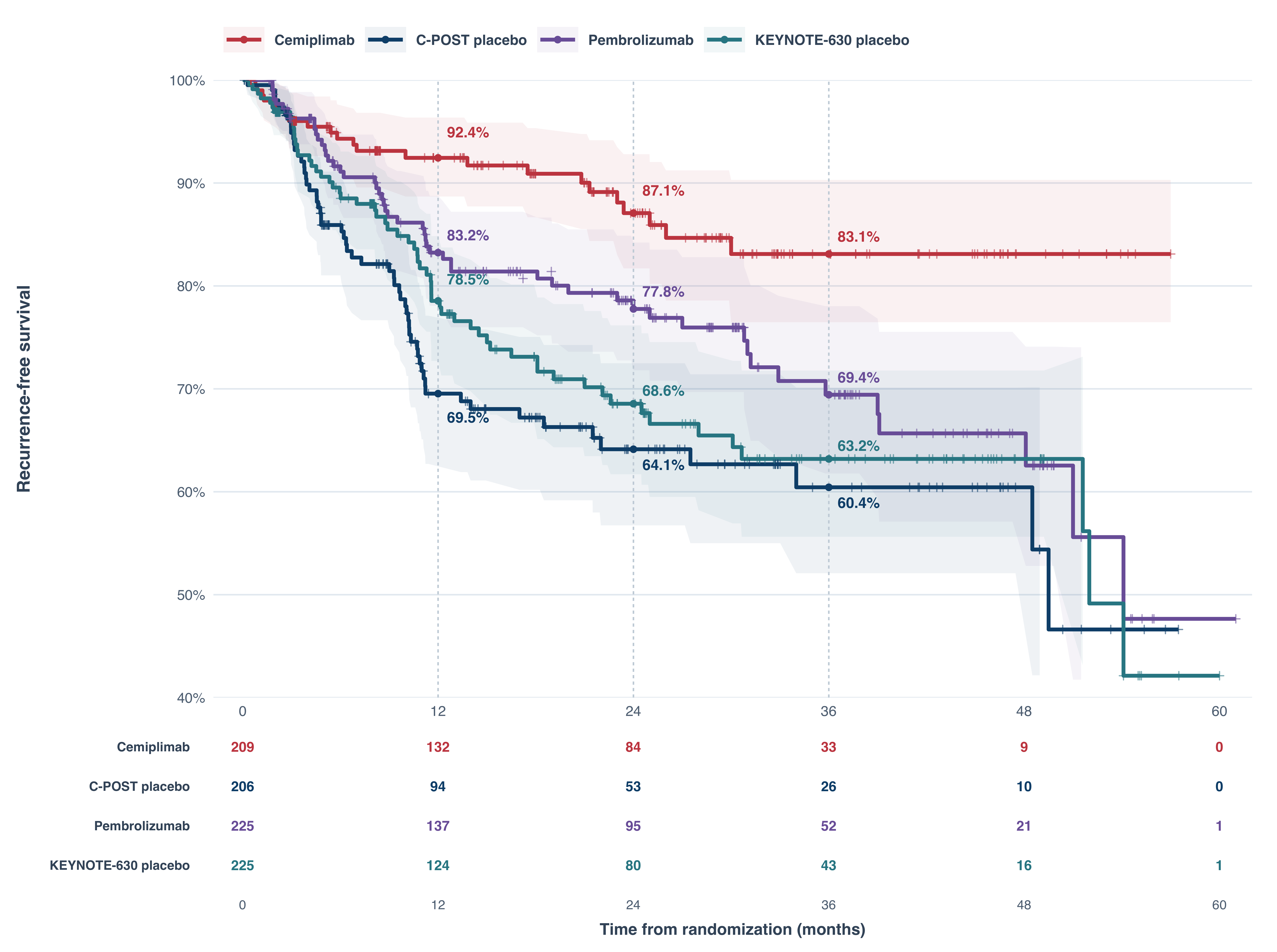
Figure 10. Reconstructed recurrence-free survival across active-treatment and placebo arms in C-POST and KEYNOTE-630. The curves are derived from pseudo–individual patient data and are presented for contextual comparison rather than as a formal cross-trial treatment analysis.
It is critical to emphasize that these reconstructed curves are intended to provide contextual insight and do not replace individual patient data meta-analysis or matching-adjusted indirect comparisons. Notably, the KEYNOTE-630 data have been presented only in abstract and conference format22 and are not yet available in a peer-reviewed manuscript. As such, many details regarding trial methodology, event ascertainment, and data maturity remain limited. These reconstructions do not adjust for imbalances in patient characteristics and cannot account for potential confounding or effect modification. Furthermore, differences in trial conduct, operational details, and the diverse centers, investigators, and care teams involved all could have contributed meaningfully to divergent outcomes.
In addition to trial-level differences, some participants raised the possibility that treatment-level factors may have influenced results. While most considered biologic differences between cemiplimab and pembrolizumab unlikely—given their similar mechanisms of action and the relatively similar published response data in unresectable CSCC—differences in dosing strategy were noted. In C-POST, an amendment to the study protocol (implemented mid-trial) introduced a shift from a fixed Q3W regimen to an induction-maintenance schedule: 350 mg Q3W for 12 weeks, followed by 700 mg Q6W for the remaining 36 weeks. In an exploratory subgroup analysis, patients treated under the revised Q6W dosing strategy had a disease-free survival hazard ratio of 0.25 (95% CI, 0.14–0.45) compared to placebo, whereas those who remained on the original Q3W-only schedule had an HR of 0.44 (95% CI, 0.18–1.09). By contrast, KEYNOTE-630 employed a fixed Q3W dosing strategy throughout. Whether these differences in scheduling contributed meaningfully to clinical outcomes remains uncertain but represents an area of interest for future study.
Timing and Its Consequences
There was also discussion about whether timing of therapy initiation may have influenced outcomes. In C-POST, the protocol initially required patients to be randomized within 2 to 6 weeks following completion of adjuvant radiation, later amended to allow up to 10 weeks. Even with this extension, the reported median time from definitive therapy to randomization was only 1.3 months, suggesting that most patients initiated systemic therapy within a relatively narrow perioperative window. By contrast, KEYNOTE-630 allowed enrollment up to 16 weeks post-radiation. While the timing distribution in KEYNOTE-630 has not been published, the broader window raises the possibility that some patients may have begun immunotherapy after early subclinical progression had already occurred.
This distinction could have both biological and statistical implications. From a biological standpoint, high-risk CSCC is known to recur early in a subset of patients, and delays in systemic therapy may allow micrometastatic disease to escape immune-mediated eradication. As illustrated in the ASCO 2025 presentation of KEYNOTE-630, more than half of locoregional failures in the placebo arm occurred within the first 6 months (30 of 57), with nearly 35% occurring by 3 months (20 of 57)22. If patients in KEYNOTE-630 initiated therapy several weeks later than in C-POST, it is plausible that the therapeutic window to prevent early recurrence had already closed in some cases. This possibility, as previously noted, hinges on the still-unproven assumption that earlier treatment of microscopic disease improves outcomes in CSCC—a biologically plausible concept that remains unconfirmed.
Statistically, early recurrences—particularly those occurring shortly after randomization but before the full effect of adjuvant therapy can manifest—can blunt the observed benefit on Kaplan–Meier curves. Because early events shape the survival curve from the outset, they can disproportionately influence time-to-event estimates and obscure true treatment effects—particularly when therapy is delayed or inconsistently timed. A more tightly controlled randomization-to-treatment window, as in C-POST, may have mitigated this effect. By contrast, greater variability in KEYNOTE-630 could have introduced bias, making it harder to detect a benefit even if one existed.
Chance, Comorbidities, and Other Unmeasured Influences
There was concern that non–cancer-related mortality—such as deaths from comorbid conditions or COVID during trial conduct—may have influenced overall survival outcomes, particularly in CSCC, where patients tend to be older. However, because most events were recurrences, not deaths, the impact of unrelated mortality on study results was likely modest. Still, in relatively small trials, even a handful of events—whether recurrences or deaths—can widen confidence intervals and complicate interpretation. All of these possibilities remain speculative in the absence of individual patient-level data.
Moving Beyond the Binary: A Bayesian Perspective
While much of the discussion has focused on the apparent contradiction between C-POST and KEYNOTE-630, it’s important to recognize that these trials are not truly in opposition – that is, one trial demonstrating efficacy and the other demonstrating no efficacy. In fact, KEYNOTE-630 demonstrated a hazard ratio point estimate that still favored anti–PD-1 therapy for locoregional and distant recurrences (HR 0.76), albeit with greater uncertainty and wider confidence intervals (95% CI 0.53-1.10; p= 0.07243), resulting in failure to achieve statistical significance22. Rather than viewing each trial in isolation or as fundamentally discordant, a more integrative perspective may offer a fuller and more accurate picture of the treatment effect.
At the root of this perceived contradiction lies a deeper statistical issue: the dominant use of frequentist statisticsb—specifically, the Neyman-Pearson decision-theoretic framework23—for interpreting clinical trial results. This framework, which underpins most regulatory decisions, including those by the FDA24, is designed to control Type I and Type II error rates across repeated sampling. It enables clear “go/no-go” decision thresholds based on p-values and pre-specified alpha levels, typically set at 0.05.
While the frequentist approach has undeniable utility—particularly in regulatory environments where long-term error control is essential—it can also promote binary interpretations of complex evidence. A trial that crosses the threshold for statistical significance is often labeled “positive,” while one that does not is deemed “negative,” even if the estimated treatment effect is clinically meaningful or directionally consistent. As a result, clinicians and stakeholders may infer divergent biological implications from what are, in fact, probabilistically overlapping results.
This binary framing can obscure the continuum of uncertainty and reinforce artificial distinctions between studies that may share more common ground than is immediately apparent. It can also lead to overinterpretation of trial outcomes as reflecting inherent differences in drug efficacy or mechanism of action—when, in reality, differences may stem from trial design, patient populations, timing of treatment, or chance.
Bayesian Synthesis: A More Integrative View
To examine the apparently discordant trial results through a different inferential framework, we performed an exploratory Bayesian evidence synthesisc, using the C-POST treatment-effect distribution as an informative prior and reconstructed KEYNOTE-630 data as the likelihood. This analysis assumes that the treatment effects observed with cemiplimab and pembrolizumab are sufficiently exchangeable across trials to permit Bayesian updating—an assumption that cannot be established from the available aggregate data. It also does not adjust for cross-trial differences in patient characteristics, eligibility, endpoint assessment, follow-up, or other study-level factors and should not be interpreted as a formal indirect comparison or as an estimate of a class-wide anti–PD-1 effect. The analysis was intended to generate and contextualize hypotheses about the apparent discordance between the trials, rather than to provide confirmatory evidence.
Under these assumptions, incorporation of the KEYNOTE-630 likelihood attenuated the larger treatment effect observed in C-POST but yielded a posterior distribution that remained below the null (Figures 11–12; posterior HR 0.56, 95% CrI 0.41–0.75). We view this result as an illustration of how the two datasets can be probabilistically reconciled, rather than evidence that resolves the discrepancy between the trials.
NoteFigure 11. Bayesian RFS: C-POST and KEYNOTE-630
Show Code Used For Bayesian Synthesis
# 🔹 Step 1: Prepare and Label Data
# Prepare analysis dataset from reconstructed survival curves
# `rfs_data_combined` is the combined patient-level survival data reconstructed
# from the Kaplan-Meier curves of the C-POST and KEYNOTE-630 trials.

df_bayes_all <- rfs_data_combined %>%
  mutate(
    # Create a new variable to classify treatment arms into anti–PD-1 or placebo
    arm_class = case_when(
      trt %in% c("Cemiplimab", "Pembrolizumab") ~ "anti_pd1",
      trt %in% c("CPOST Placebo", "KN630 Placebo") ~ "placebo"
    ),

    # Create a new variable to indicate which trial each arm belongs to
    trial = case_when(
      trt %in% c("Cemiplimab", "CPOST Placebo") ~ "CPOST",
      trt %in% c("Pembrolizumab", "KN630 Placebo") ~ "KN630"
    )
  ) %>%
  filter(!is.na(arm_class))  # Keep only rows with valid treatment classification

# Set placebo as reference level
df_combined <- df_bayes_all %>%
  mutate(arm_class = relevel(factor(arm_class), ref = "placebo"))

# 🔹 Step 2: Model C-POST as Prior
df_prior <- df_bayes_all %>% filter(trial == "CPOST")

# Fit Bayesian Cox model to estimate prior from C-POST
fit_prior <- brm(
  # Specify the model formula:
  # `time` is the observed survival time
  # `event` is the event indicator (1 = event occurred, 0 = censored)
  # `cens(1 - event)` tells brms which values are censored (i.e., 1 - event == 1 means censored)
  # `~ arm_class` compares anti–PD-1 vs placebo groups
  formula = brmsformula(time | cens(1 - event) ~ arm_class),

  # Use only the C-POST data to inform the prior
  data = df_prior,

  # Specify that this is a Cox proportional hazards model
  # `brmsfamily("cox")` sets the survival model type
  family = brmsfamily("cox"),

  # Define the prior distribution:
  # Apply a Normal(0, 1) prior to the log hazard ratio (HR) coefficient
  # This reflects moderate prior certainty that log(HR) is near 0 (i.e., HR ≈ 1),
  # but allows for moderate deviations
  prior = prior(normal(0, 1), class = "b"),

  # Run 4 Markov chains to ensure robust sampling
  chains = 4,

  # Each chain runs for 2000 iterations (includes warmup)
  iter = 2000,

  # Use 4 cores to parallelize the model fitting
  cores = 4,

  # Set a fixed random seed for reproducibility
  seed = 123
)

# Extract log HR distribution to use as prior in synthesis
prior_draws <- fit_prior %>%
  spread_draws(b_arm_classplacebo) %>%
  mutate(logHR = -b_arm_classplacebo)

logHR_mean <- mean(prior_draws$logHR)
logHR_sd   <- sd(prior_draws$logHR)
# Summarize HR from prior
hr_prior <- prior_draws %>%
  mutate(HR = exp(logHR)) %>%
  summarise(
    source = "Prior (C-POST)",
    HR_median = median(HR),
    HR_CI_low = quantile(HR, 0.025),
    HR_CI_high = quantile(HR, 0.975)
  )
# 🔹 Step 3: Estimate Likelihood from KN630
df_likelihood <- df_bayes_all %>% filter(trial == "KN630")

fit_likelihood <- brm(
  # Specify the model formula:
  # We are modeling survival time (`time`) using a Cox proportional hazards model.
  # `cens(1 - event)` indicates censoring: when `event` is 0, the observation is censored.
  # The predictor is `arm_class`, comparing anti–PD-1 vs placebo.
  formula = brmsformula(time | cens(1 - event) ~ arm_class),

  # Provide the dataset for this model: KN630 trial observations only.
  # Also ensure the `arm_class` factor is explicitly re-leveled
  # so that "placebo" is treated as the reference level (HR < 1 favors anti–PD-1).
  data = df_likelihood %>%
    mutate(arm_class = relevel(factor(arm_class), ref = "placebo")),

  # Specify the model family: a Cox proportional hazards model for time-to-event data
  family = brmsfamily("cox"),

  # Set a weakly informative prior: Normal(0, 5) on the log hazard ratio.
  # This allows for a wide range of plausible treatment effects, reflecting limited prior knowledge.
  prior = prior(normal(0, 5), class = "b"),  # "b" refers to regression coefficients

  # Use 4 Markov chains:
  # In Bayesian inference, Markov Chain Monte Carlo (MCMC) is used to sample from the posterior distribution.
  # Running multiple chains helps diagnose convergence and avoid local optima.
  chains = 4,

  # Set the number of iterations per chain:
  # 2000 iterations per chain (including warmup), giving a total of ~8000 samples.
  iter = 2000,

  # Run the chains in parallel using 4 processor cores
  cores = 4,

  # Set a seed for reproducibility
  seed = 123
)

hr_likelihood <- fit_likelihood %>%
  spread_draws(b_arm_classanti_pd1) %>%
  mutate(HR = exp(b_arm_classanti_pd1)) %>%
  summarise(
    source = "Likelihood (KEYNOTE-630)",
    HR_median = median(HR),
    HR_CI_low = quantile(HR, 0.025),
    HR_CI_high = quantile(HR, 0.975)
  )
# 🔹 Step 4: Fit Combined Model Using Informative Prior
fit_combined <- brm(
  formula = brmsformula(
    time | cens(1 - event) ~ arm_class # “Fit a Bayesian survival model for time, accounting for censoring, with arm_class as the predictor.”
    ),
  data = df_combined %>% filter(trial == "KN630"),
  family = brmsfamily("cox"),
  prior = prior_string( # Informative prior in synthesis step:
    paste0("normal(", logHR_mean, ", ", logHR_sd, ")"),
    class = "b" # "b" stands for "beta", which represents the coefficients for predictors in the model (e.g., treatment arm); class = "b" tells brms to apply the prior to the log hazard ratio for the treatment effect.
  ),
  chains = 4, iter = 2000, cores = 4,
  seed = 123
)
# Summarize posterior
hr_posterior <- fit_combined %>%
  spread_draws(b_arm_classanti_pd1) %>%
  mutate(HR = exp(b_arm_classanti_pd1)) %>%
  summarise(
    source = "Posterior (Synthesis)",
    HR_median = median(HR),
    HR_CI_low = quantile(HR, 0.025),
    HR_CI_high = quantile(HR, 0.975)
  )
# 🔹 Final: Combine and Plot Summary
# Combine results
hr_summary <- bind_rows(hr_prior, hr_likelihood, hr_posterior)

# Posterior from your BRMS model (e.g., posterior synthesis)
posterior_draws <- as_draws_df(fit_combined)
beta <- posterior_draws$b_arm_classanti_pd1

# 🔧 Step 1: Fit Frequentist Cox Model (for baseline hazard)
# Fit survival model to get baseline hazard
fit_km <- coxph(Surv(time, event) ~ arm_class, data = df_bayes_all)

# Extract baseline cumulative hazard (for placebo group)
base_haz <- basehaz(fit_km, centered = FALSE) # Shared baseline hazard is from:
base_haz <- base_haz %>%
  rename(
    time = time,
    cumhaz = hazard
    ) # A piecewise exponential model assumes constant hazard in small intervals. While brms does not natively label this as “piecewise exponential,” when you extract the baseline cumulative hazard from coxph and apply it in a discrete-time grid as done here, you are essentially approximating a piecewise exponential function over those time intervals.

# 🔁 Step 2: Extract Posterior Coefficients

# Posterior from your BRMS model (e.g., posterior synthesis)
posterior_draws <- as_draws_df(fit_combined)
beta <- posterior_draws$b_arm_classanti_pd1 # Treatment-specific effect is incorporated via this code

# 📈 Step 3: Simulate Survival Curves

# Expand basehaz for both arms and apply survival formula
# Simulate survival curves for each draw of beta (anti-PD1 arm)
surv_draws <- map_dfc(seq_along(beta), function(i) {
  exp(-base_haz$cumhaz * exp(beta[i]))
}) # This applies the exponential survival function over time using posterior draws of the treatment effect (beta[i]), yielding smooth survival curves.

# Rename columns
names(surv_draws) <- paste0("draw_", seq_along(beta))

# Assemble into one dataframe
surv_df <- bind_cols(
  base_haz %>% select(time, cumhaz),
  surv_placebo = exp(-base_haz$cumhaz),
  surv_draws
)

# Summarize median + 95% CI
## This aggregates survival probabilities across 2000+ draws for each time point — producing posterior median curves with 95% credible intervals, as plotted.
surv_summary <- surv_df %>%
  select(time, starts_with("draw_")) %>%
  pivot_longer(cols = starts_with("draw_"), names_to = "draw", values_to = "surv") %>%
  group_by(time) %>%
  summarise(
    median = median(surv),
    lower = quantile(surv, 0.025),
    upper = quantile(surv, 0.975),
    .groups = "drop"
  ) %>%
  mutate(arm_class = "anti–PD1")

# Add placebo line
placebo_df <- surv_df %>%
  select(time, surv_placebo) %>%
  rename(median = surv_placebo) %>%
  mutate(
    lower = median,
    upper = median,
    arm_class = "Placebo"
  )


# Combine and plot
plot_data <- bind_rows(
  surv_summary %>% select(time, median, lower, upper, arm_class),
  placebo_df %>% select(time, median, lower, upper, arm_class)
)
# Filter to posterior synthesis
hr_row <- hr_summary %>%
  filter(source == "Posterior (Synthesis)")

# Create HR annotation text
hr_text <- glue(
  "HR: {round(hr_row$HR_median, 2)} ",
  "(95% CI: {round(hr_row$HR_CI_low, 2)}–{round(hr_row$HR_CI_high, 2)})"
)
hr_text

p_bayes <-
  ggplot(
    plot_data,
    aes(x = time, y = median, color = arm_class, fill = arm_class)) +
  geom_line(size = 1.2) +
  geom_ribbon(aes(ymin = lower, ymax = upper), alpha = 0.2, color = NA) +
  geom_vline(
    xintercept = c(12, 24, 36),
    linetype = "dashed", color = "black") +
  labs(
    title = "Posterior Recurrence-Free Survival",
    subtitle = "Bayesian Synthesis of CPOST and KN630",
    x = "Time (Months)",
    y = "Estimated Survival Probability",
    color = "",
    fill = ""
  ) +
  scale_y_continuous(
    labels = scales::percent_format(accuracy = 1),
    breaks = seq(0, 1, by = 0.1),
    limits = c(0, 1)
  ) +
  scale_color_manual(values = c("Placebo" = "#377EB8", "anti–PD1" = "#E41A1C")) +
  scale_fill_manual(values = c("Placebo" = "#377EB8", "anti–PD1" = "#E41A1C")) +
  theme_minimal(base_size = 14) +
  theme(
    plot.title = element_text(size = 20, face = "bold", hjust = 0.5),
    plot.subtitle = element_text(size = 16, face = "bold", hjust = 0.5),
    axis.title = element_text(size = 16),
    axis.text = element_text(size = 14),
    legend.position = "none"
  )

p_bayes

p_bayes <- p_bayes +
  scale_x_continuous(
    breaks = seq(0, 60, by = 6),
    limits = c(0, 66)
  )

p_bayes
# If you want to add % survival labels at specific time points
annot_df <- plot_data %>%
  group_by(arm_class) %>%
  slice_min(abs(time - 12), n = 1) %>%
  bind_rows(
    plot_data %>% group_by(arm_class) %>% slice_min(abs(time - 24), n = 1),
    plot_data %>% group_by(arm_class) %>% slice_min(abs(time - 36), n = 1)
  ) %>%
  mutate(
    label = paste0(round(median * 100, 1), "%"),
    vjust = ifelse(arm_class == "Placebo", 1.8, -0.6)
  )

p_bayes <- p_bayes +
  geom_text(
    data = annot_df,
    aes(label = label),
    size = 5,
    fontface = "bold",
    hjust = -0.3,
    vjust = annot_df$vjust
  )

p_bayes

end_labels <- plot_data %>%
  group_by(arm_class) %>%
  filter(time == max(time)) %>%
  mutate(y_pos = median + ifelse(arm_class == "Placebo", 0.03, -0.03))

p_bayes <- p_bayes +
  geom_text(
    data = end_labels,
    aes(
      x = time - 2,
      y = y_pos,
      label = arm_class, color = arm_class),
    fontface = "bold",
    size = 5
  )
p_bayes


p_bayes <- p_bayes +
  annotate(
    "text",
    x = Inf, y = -Inf,
    label = hr_text,
    hjust = 1.05,
    vjust = -1.5,
    size = 4.5,
    fontface = "bold"
  )
p_bayes


# Time points of interest
time_points <- seq(0, 60, by = 6)

# Function to count number at risk at each time per arm
risk_table <- df_bayes_all %>%
  mutate(time = floor(time)) %>%
  group_by(arm_class, time) %>%
  summarise(
    n_risk = sum(time >= unique(time_points)),
    .groups = "drop") %>%
  filter(time %in% time_points)

risk_table <- purrr::map_dfr(time_points, function(t) {
  df_bayes_all %>%
    filter(time >= t) %>%
    count(arm_class) %>%
    mutate(time = t)
  })

risk_plot <-
  ggplot(risk_table, aes(x = time, y = arm_class, label = n)) +
  geom_text(size = 5) +
  scale_x_continuous(breaks = time_points) +
  scale_y_discrete(
    labels = c("placebo" = "Placebo", "anti_pd1" = "Anti–PD1")) +  # 👈 manually set label
  labs(
    x = "Time (Months)",
    y = NULL,
    title = "Number at Risk"
  ) +
  theme_minimal(base_size = 16) +
  theme(
    axis.text.y = element_text(face = "bold"),
    panel.grid.major.y = element_blank(),
    plot.title = element_text(hjust = 0.5, face = "bold")
  )

final_plot <- p_bayes / risk_plot + plot_layout(heights = c(3, 1))
print(final_plot)
Bayesian evidence synthesis
The posterior supports a consistent anti–PD-1 treatment effect.
C-POST informs the prior; reconstructed KEYNOTE-630 data update the evidence to produce posterior recurrence-free survival estimates.
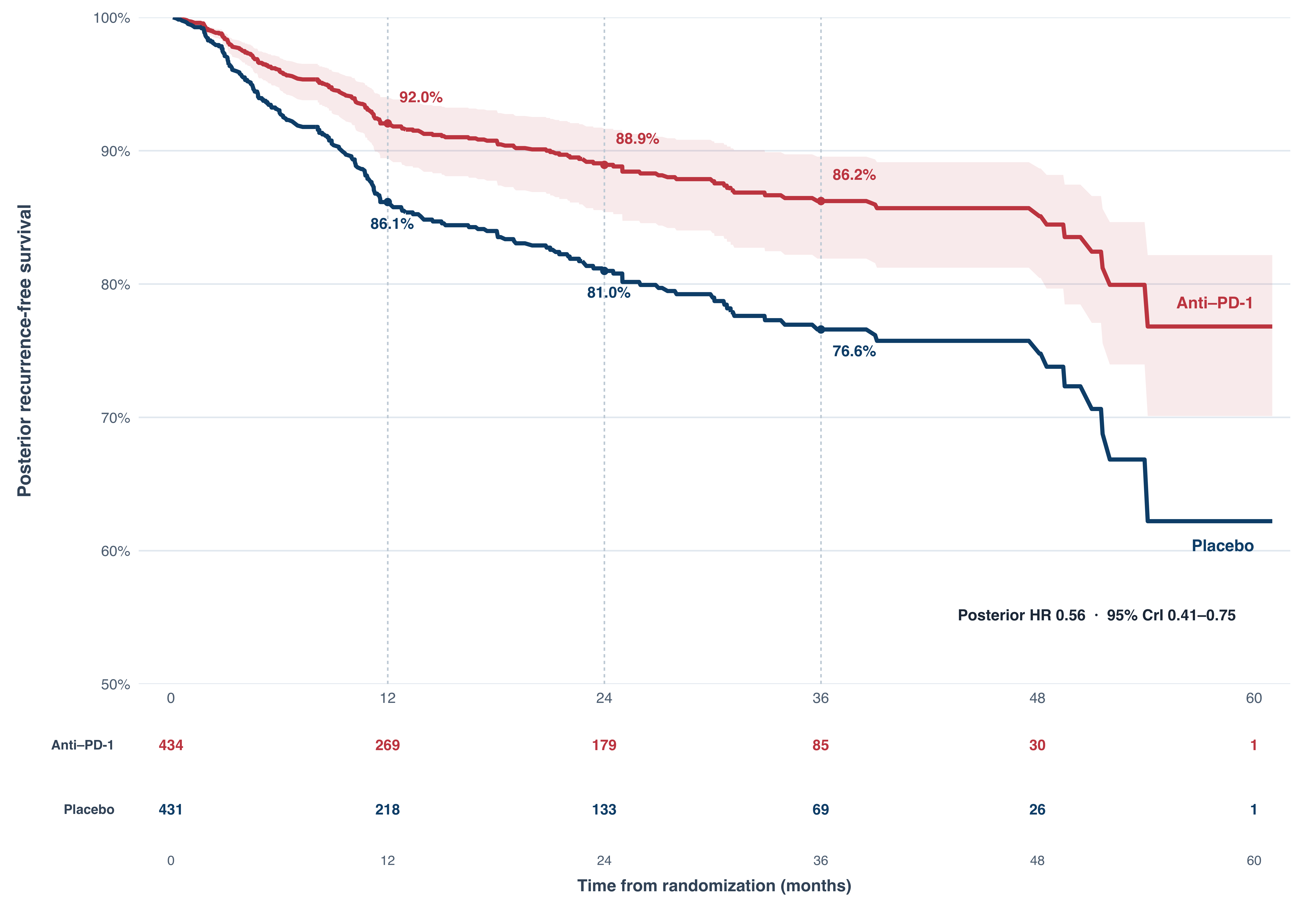
Figure 11. Posterior recurrence-free survival after Bayesian synthesis of C-POST and reconstructed KEYNOTE-630 evidence. C-POST was used to inform the prior treatment-effect distribution, which was then updated with KEYNOTE-630 pseudo–individual patient data; the posterior hazard ratio for anti–PD-1 versus placebo was 0.56 (95% CrI, 0.41–0.75). The curves are model-based posterior estimates and should be interpreted as an evidence synthesis rather than pooled randomized patient-level data.
NoteFigure 12. Bayesian Forest Plot: Anti–PD-1 vs Placebo
Show Code Used For Forest Plot
# Prepare summary data for plotting the prior, likelihood, and posterior hazard ratios
# This tibble reflects the results from the Bayesian models constructed in Figure 11.
# Each row corresponds to a step in the Bayesian synthesis:
#   - "Prior (C-POST)" comes from the model fit to the C-POST trial data alone
#   - "Likelihood (KEYNOTE-630)" reflects the model fit to KEYNOTE-630 data
#   - "Posterior (Synthesis)" is the updated estimate after combining the two using Bayesian inference

hr_summary <- tibble::tibble(
  source = factor(
    c("Prior (C-POST)", "Likelihood (KEYNOTE-630)", "Posterior (Synthesis)"),
    levels = rev(c("Prior (C-POST)", "Likelihood (KEYNOTE-630)", "Posterior (Synthesis)"))
  ),
  HR_median = c(0.337, 0.767, 0.556),
  HR_CI_low = c(0.207, 0.531, 0.414),
  HR_CI_high = c(0.530, 1.11, 0.748)
)

# Plot
forest_bayes <-
  ggplot(hr_summary, aes(x = HR_median, y = source)) +
  geom_point(size = 3) +
  geom_errorbarh(aes(xmin = HR_CI_low, xmax = HR_CI_high), height = 0.2) +
  geom_vline(xintercept = 1, linetype = "dashed", color = "gray40") +
  labs(
    title = "Bayesian Synthesis of HR for Anti–PD-1 vs Placebo",
    x = "Hazard Ratio (HR)",
    y = NULL
  ) +
  theme_minimal(base_size = 18)

forest_bayes
Bayesian treatment-effect update
The posterior lands between C-POST and KEYNOTE-630.
C-POST provides the prior treatment-effect distribution; the reconstructed KEYNOTE-630 estimate updates that evidence to yield the posterior hazard ratio.
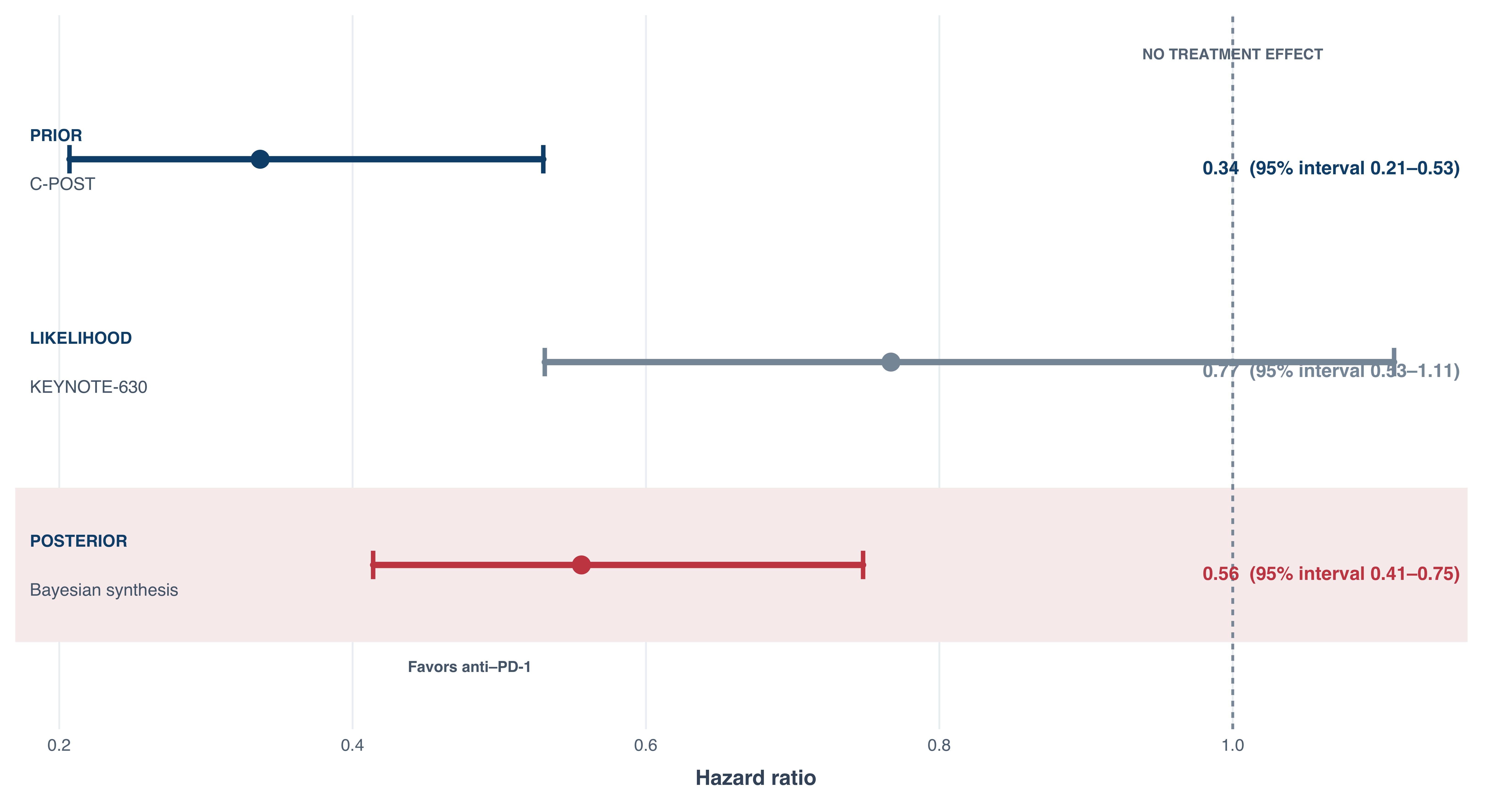
Figure 12. Bayesian update of the recurrence-free survival hazard ratio for anti–PD-1 therapy versus placebo. C-POST informs the prior, reconstructed KEYNOTE-630 provides the likelihood, and the resulting posterior estimate is HR 0.56 (95% CrI, 0.41–0.75).
The purpose of this synthesis is not to collapse C-POST and KEYNOTE-630 into a single definitive estimate or to explain away their different primary outcomes. Rather, it illustrates that the two studies need not be viewed as biologically incompatible: under the assumptions used here, the KEYNOTE-630 data attenuate—but do not necessarily erase—the treatment-effect distribution informed by C-POST. Why the trials differed remains unresolved and may reflect patient selection, trial design, treatment differences, chance, or some combination of these factors.
Conclusion
C-POST represents a major advance in the perioperative management of CSCC, positioning immunotherapy—and cemiplimab in particular—as a new standard alongside or even ahead of radiation. Still, it does not settle whether immune checkpoint blockade should be applied routinely across all patients with resectable high-risk disease. The failure of KEYNOTE-630 to achieve statistical significance and ongoing concerns about overtreatment underscore the need for careful implementation. As the field continues to evolve, longer follow-up, cancer-specific outcomes, and additional randomized or real-world data will be essential to guide more precise patient selection and optimize benefit.
Materials and Methods
Bibliography
Article Information
NoteArticle Details
Abbreviations
Adj, adjuvant; APP, advanced practice provider; ART, adjuvant radiation therapy; CI, confidence interval; CrI, credible interval; CSCC, cutaneous squamous cell carcinoma; DFS, disease-free survival; ECE, extracapsular extension; ECOG, Eastern Cooperative Oncology Group; FDA, U.S. Food and Drug Administration; GEP, gene expression profile; ICI, immune checkpoint inhibitor; IPD, individual patient data; LN, lymph node; MDC, multidisciplinary clinic; Med, medical; NCCN, National Comprehensive Cancer Network; NED, no evidence of disease; Neo, neoadjuvant; NeoAdj, neoadjuvant; NMSC, nonmelanoma skin cancer; Path Eval, pathologic evaluation after surgery; PD-1, programmed death-1; PMH, past medical history; Post-op, postoperative; Q3W, every three weeks; Q6W, every six weeks; RFS, recurrence-free survival; RT, radiation therapy; SC, subcutaneous; SoCO, Society of Cutaneous Oncology; Surg, surgical; Tx, treatment; UnTx, untreated.
Acknowledgments
We also wish to acknowledge the following individuals from Regeneron for their participation in the Journal Club discussion and for sharing helpful insights regarding the development and interpretation of the C-POST study: Christopher Zajac, Alyson Baryiames, Sarah Nia, Brian Burleson, Kim Premo, Frank Seebach, Julie Montiel, and Matthew Fury.
Citation
For attribution, please cite this work as:
Miller DM, Patel VA, Sondak VK, Tchekmedyian V, Merkin RD, Brownell I, Drews RE, Gupta S, Khushalani NI, Nghiem PT, Kaufman HL, Emerick KS. Evolving Standards for Resected High-Risk CSCC: Integrating Insights from C-POST and KEYNOTE-630. Journal of Cutaneous Oncology. 2025;3(2). https://doi.org/10.59449/joco.2025.09.03 Copied!
BibTeX citation:
@article{miller,
  author = {Miller, David M. and Patel, Vishal A. and Sondak, Vernon K. and Tchekmedyian, Vatche and
          Merkin, Ross D. and Brownell, Isaac and
          Drews, Reed E. and Gupta, Sameer and Khushalani, Nikhil I. and
          Nghiem, Paul T. and Kaufman, Howard L. and Emerick, Kevin S.},
  title = {Evolving Standards for Resected High-Risk CSCC: Integrating Insights from C-POST and KEYNOTE-630},
  journal = {Journal of Cutaneous Oncology},
  volume = {3},
  number = {2},
  url = {https://journalofcutaneousoncology.io/perspectives/Vol_3_Issue_2/adjuvant_cemiplimab_for_high_risk_resected_cscc/},
  doi = {10.59449/joco.2025.09.03},
  issn = {2837-1933},
  publisher = {Society of Cutaneous Oncology},
  langid = {en}
}
Disclaimer
This site represents our opinions only. See our full Disclaimer
Disclosures
Conflict of Interests
Dr. Miller has received honoraria for serving as a consultant or participation on advisory boards for Almirall, Bristol Myers Squibb, Merck, EMD Serono, Regeneron, Sanofi Genzyme, Pfizer, Castle Biosciences, Checkpoint Therapeutics and Sun Pharmaceuticals. He serves on the Unloxcyt steering committee for Sun Pharmaceuticals. He has stock options from Avstera Therapeutics. He has received institutional research funding from Regeneron, Kartos Therapeutics. NeoImmune Tech, Inc, Project Data Sphere, ECOG-ACRIN and the American Skin Association. Dr. Khushalani owns stock in Amarin Pharma Inc., Asensus Surgical, and Bellicum Pharmaceuticals. He participates in data and safety monitoring for AstraZeneca and Incyte Corporation. He has served as a consultant for Bristol Myers Squibb, Castle Biosciences, Genzyme, Immunocore, Instil Bio, IO Biotech, Iovance Biotherapeutics, Jounce, Merck, Mural Oncology, MyCareGorithm, Nektar, Novartis, Regeneron Pharmaceuticals, Replimune, T-Knife Therapeutics, Delcath and Sun Pharmaceuticals. Dr. Nghiem reports compensation/support from UpToDate (honoraria), Almirall (advisory role), Incyte (institutional research funding), and has a patent pending for high-affinity T-cell receptors that target the Merkel polyomavirus, Patent filed: “Merkel cell polyomavirus T antigen-specific TCRs and uses thereof” (institution). Dr. Kaufman is an employee of Ankyra Therapeutics. He has served in advisory roles for Castle Biosciences, Marengo Therapeutics, Tatum Biosciences, and Virogin Biotech; serves on the Board of Crichton Biosciences; holds stock in Replimune, Inc.; and has received honoraria from the Society for Immunotherapy of Cancer. Dr. Sondak is a compensated consultant for Bristol Myers Squibb, Merck, and Mural Oncology, and receives research funding from Neogene Therapeutics and Skyline. Drs. Tchekmedyian, Merkin, Brownell, and Drews report no relevant disclosures.
Endnotes
a. What Is Pseudo–Individual Patient Data? When individual patient data from a clinical trial are not publicly available, researchers can approximate them using a method called pseudo–individual patient data (IPD) reconstruction. This technique uses published Kaplan–Meier survival curves and the associated number-at-risk tables to estimate the time-to-event outcomes for each participant.
Think of it as reverse-engineering the survival curve: by digitizing the graph and combining it with tabular data, we can simulate a realistic, though imperfect, version of the underlying dataset. This approach allows exploratory comparisons across trials and supports hypothesis generation—even in the absence of raw data.
Limitations remain: these estimates cannot fully replicate the original dataset and do not adjust for confounding variables. But they offer a valuable tool for contextualizing trial results when patient-level data are unavailable.
b. Frequentist vs. Bayesian Thinking. Frequentist inference—the traditional framework used in most clinical trials and regulatory decisions—interprets probability as long-run frequency. A p-value reflects the probability of observing results as extreme as the data, assuming the null hypothesis is true. Decisions are made using fixed thresholds (e.g., p < 0.05), optimizing control of long-term Type I and II errors.
Bayesian inference, by contrast, interprets probability as a degree of belief. It combines prior knowledge (from earlier studies or clinical judgment) with new data (likelihood) to generate a posterior distribution—a full, updated estimate of effect with direct probabilistic interpretation (e.g., “there is a 95% probability the hazard ratio is less than 1”).
Key difference: Frequentist results emphasize statistical significance, while Bayesian results emphasize evidence updating. Both have value, but Bayesian models may better reflect how clinicians reason under uncertainty and incorporate external knowledge.
c. Bayesian Synthesis. At a high level, a Bayesian synthesis is a way of combining prior knowledge with new information to form an updated conclusion. In this case, we used the results from one clinical trial (C-POST) as our “starting belief” (called the prior), and then incorporated data from a second trial (KEYNOTE-630) to revise that belief. The term likelihood refers to how well the new data align with different possible effects of the treatment. When we combine the prior and the likelihood, we arrive at what’s called the posterior estimate—a refined, updated estimate that reflects both sets of evidence.
This approach is grounded in Bayes’ Theorem, which provides a formal framework for updating beliefs in light of new data. In doing so, it enables us to learn iteratively and transparently, especially in settings where direct evidence may be limited or evolving.
License
This work is licensed under a creative commons BY-NC-ND license

Publication Stage
- Published